DEMOGRAPHIC RESEARCH
A peer-reviewed, open-access journal of population sciences
DEMOGRAPHIC RESEARCH
VOLUME 37, ARTICLE 57, PAGES 1825–1860
PUBLISHED 08 DECEMBER 2017
http://www.demographic-research.org/Volumes/Vol37/57/ DOI: 10.4054/DemRes.2017.37.57
Research Article
The empirical content of season-of-birth
effects: An investigation with Turkish data
Huzeyfe Torun
Semih Tumen
c
2017 Huzeyfe Torun & Semih Tumen.
This open-access work is published under the terms of the Creative Commons Attribution 3.0 Germany (CC BY 3.0 DE), which permits use, reproduction, and distribution in any medium, provided the original author(s) and source are given credit.
1 Introduction 1826
2 Data 1829
3 Empirical analysis and discussion 1830
3.1 Season-of-birth patterns in Turkey 1830
3.2 Potential drivers of the season-of-birth patterns 1833
3.3 Education and labor market outcomes 1835
3.4 Parental background 1848
3.5 Implications for policy evaluation 1850
4 Concluding remarks 1854
The empirical content of season-of-birth effects:
An investigation with Turkish data
Huzeyfe Torun1
Semih Tumen2
Abstract
BACKGROUND
Our aim is to investigate the link between season of birth and socioeconomic background.
OBJECTIVE
Season of birth is often used as an instrumental variable in answering various research questions in demography and economics. We use Turkish data to point out the poten-tial deficiencies of this approach. We show that these deficiencies can be amplified in developing-country settings due to measurement errors.
METHODS
We merge administrative birth records into the Turkish Labor Force survey and use OLS, IV–2SLS, and regression discontinuity approaches to answer the question we pose.
RESULTS
We find that, due to certain institutional, cultural, and geographical factors, around 20% of the Turkish population are reported to have been born in January. Moreover, January-born individuals have, on average, a worse socioeconomic background than individuals born in other months.
CONCLUSIONS
These findings suggest that the season-of-birth variable, which is used as an instrumental variable (IV) in many studies using Turkish data, is not random; thus, one should be careful in implementing IV estimation based on season-of-birth cutoffs. In particular, it cannot be used in regression discontinuity exercises relying on date cutoffs around January 1 (which important policy efforts such as the reform of compulsory education often do) unless handled with caution.
1Structural Economic Research Department, Central Bank of the Republic of Turkey, Ankara, Turkey.
E-Mail:[email protected].
2Structural Economic Research Department, Central Bank of the Republic of Turkey, Ankara, Turkey.
CONTRIBUTION
The main contribution of this paper is to show that the season-of-birth variable is poten-tially nonrandom (i.e., it is not independent from family background) for several reasons, and the degree of this nonrandomness is likely amplified in developing-country settings.
1. Introduction
The interaction between season-birth patterns and compulsory-schooling laws is of-ten used in the labor economics literature to construct an instrumental variable (IV) for the purpose of estimating the causal impact of education on earnings (see, e.g., Angrist and Krueger 1991). Several countries, including the United States, have compulsory-schooling laws that keep young individuals enrolled in school until a certain age – typ-ically until their 15thor 16thbirthdays. Given this restriction, the season-of-birth differ-entials across individuals generate exogenous variation in the time spent in school for those for whom the compulsory school-leaving age is binding. This exogeneity is strictly conditional on the assumption that the season of birth is not a choice made by the parents or it is not systematically correlated with parental background.
However, there is no consensus in the literature on the validity of this exogeneity assumption. Papers including Angrist and Krueger (1992, 1995, 2001), Card (1999), and Hoogerheide, Kleibergen, and van Dijk (2007) argue that the date of birth is likely random and cannot be related to one’s ability or parental background. There is a large body of empirical papers taking this argument as given and performing IV methods to estimate the returns to education.3 Another set of papers – including Bound, Jaeger, and Baker
(1995), Bound and Jaeger (2001), and Buckles and Hungerman (2013) – documents that the exogeneity condition is typically not satisfied.4
Two explanations are offered in the literature to validate the latter argument. First, richer and more educated parents are more likely to have children in the third or fourth quarters of the year. Buckles and Hungerman (2013) find that there is no seasonality in unwanted births – for example, births by teenagers and the unmarried. These women mostly have low socioeconomic status. Women of higher socioeconomic status, on the other hand, are much less likely to give birth voluntarily in winter. Therefore, seasonal patterns in fertility are mostly driven by the conception behavior of women of higher socioeconomic status. Second, the evidence suggests that winter births are subject to
3 See, e.g., Levin and Plug (1999), Plug (2001), Gelbach (2002), Hansen, Heckman, and Mullen (2004),
Skirbekk, Kohler, and Prskawetz (2004), Lefgren and McIntyre (2006), Leigh and Ryan (2008), Maurin and Moschion (2009), Lee and Orazem (2010), and Robertsen (2011).
worse outcomes due to in-utero exposure to weather and illness.5 Moreover, if nutrition is also seasonal, this could also lead to differential fetal development patterns across seasons (Barker 2001). Other studies documenting that the ones who are born early in the year are more likely to suffer from mental health problems than the ones who are born later in the year include Livingston, Adam, and Bracha (1993), Tochigi et al. (2004), and Doblhammer, Scholz, and Maier (2005). These arguments suggest that, although the idea to use season of birth as an IV idea is a solid one, the patterns of variation in the school attainment across the quarters or months of year may not be solely driven by exogenous forces. Therefore, the causal nature of the returns to schooling estimates obtained with the season of birth IV is questionable.
In this paper, we contribute to this debate by providing evidence from Turkey using a large micro-level data set with rich content related to individuals’ educational and labor market outcomes. Previous literature focuses on the uneven characteristics across seasons of birth rather than the uneven density. In our case, we start by documenting the uneven density across months of births in Turkey and then argue that this is due to misreporting behavior of parents who have lower socioeconomic status. We show that around 20% of the entire population in Turkey are registered as January-born; when we only consider individuals age 60 and above, this fraction goes up to around 35%. The tendency to misreport the birth date is a consequence of a combination of geographical, seasonal, and institutional factors. First, especially in the past, the individuals residing in rural areas might have had difficulty in commuting to city centers in the winter season to officially report the birth of their children. These children are reported after the winter season is over and their birth date is usually registered as January 1 of the corresponding year. Second, teenage marriages are more common in some regions of Turkey, and children of teenage parents are not registered immediately after the birth. These children are also generally registered as having been born in January. Finally, some parents choose to report the children who are born in October, November, and December of a given yeart as if they were born in January of yeart+ 1. The main motivation is the perception that younger children in a given cohort are less successful in school than the older ones.
Since these phenomena occur mostly in rural and less developed areas of the country, being registered as January-born is associated with worse educational and labor market outcomes. In particular, we find that January-born individuals receive around half a year less schooling than the children who are born in the other months of the year. Moreover, the January-born individuals earn around 2–5% less than others. We conclude that the season of birth, especially being January-born, predicts worse later outcomes in Turkey. Thus, we conclude that the tendency to misreport discussed above is another reason why the season of birth is not orthogonal to later outcomes. We believe that this result is not specific to Turkey. In many other cultures the birthday is registered to be January 1
if a person’s real birthday is unknown for some reason, and the reason is most likely associated with a low socioeconomic status. Even in developed countries with heavy exposure to immigrant flows, birth date statistics are plagued by misreporting, especially those of first-generation immigrants.
We also argue that our results are important for econometric policy evaluation prac-tices. Certain important policyies in Turkey, such as the compulsory-education reform and the law providing men with the option to benefit from an exemption from compulsory military service, are based on January 1 cutoff birth dates.6 Individuals born before and
after this cutoff birth date are exposed to different regulations and environments. Most importantly, the official birth dates are binding for eligibility to these reforms. Since we argue that a January-born individual in Turkey is more likely to have a weaker socioe-conomic background, the January 1 cutoff cannot be regarded as an exogenous policy reform cutoff date unless the seasonality is considered carefully. In fact, the January 1 cut-off more likely separates the ones with weaker backgrounds from the ones with stronger backgrounds. Therefore, policy evaluation methods that rely on the January 1 cutoff, such as regression discontinuity designs and IV, are highly likely to produce biased re-sults unless handled with caution. To confirm the validity of this concern, we evaluate the effectiveness of ten different placebo policy reforms with January 1 as the birth date cutoffs, and we conclude that the ones who are born in January have worse educational and labor market outcomes than the ones born in December. In other words, any ‘policy’ (whatever it is) that separates January-born from December-born individuals will lead to more favorable outcomes for the December-born. Therefore, caution should be exercised in performing the methods used to evaluate the policies with January 1 as the cutoff birth date.
In a broader sense, our paper can also be placed into the literature investigating the degree of seasonality in births across countries. The existing evidence suggests that sea-sonality of births exhibits substantial cross-country and time-series variation (Lam and Miron 1994; Dor´elien 2016). Most of the time, the underlying seasonal pattern has a behavioral explanation, including lower rates of conception during the harvest period in rural Germany (Knodel and Wilson 1981), birth avoidance during peak labor demand pe-riods in Egypt (Levy 1986), seasonal migration from Mexico to the United States (Massey and Mullan 1984), the interplay between occupational transformation and women’s en-ergy intake in Iceland (Bjornsson and Zoega forthcoming), and various reasons rang-ing from agricultural production activity to disease transmission in sub-Saharan Africa (Dor´elien 2016).7 These papers mostly focus on behavioral forces that generate season-ality in actual birth dates. There is a smaller set of papers documenting seasonseason-ality in
6See, e.g., Aydemir and Kirdar (2017), Torun (2015), Cesur and Mocan (forthcoming), and Torun and Tumen
(2016).
7More recent papers in this literature include Dickert-Conlin and Chandra (1999), Gans and Leigh (2009),
reported birth dates due to misreporting practices. Similar to our paper, Schultz-Nielsen, Tekin, and Greve (2016) also find that there are spikes in January 1 birth dates (and also July 1 to a smaller extent) among Muslims in Denmark. Dor´elien (2016) reviews the liter-ature documenting birth date misreporting practices in sub-Saharan Africa. Our paper is the first in the literature providing a full picture of birth date misreporting in a developing-country context by paying particular attention to the factors driving misreporting as well as other related statistical and economic matters.
This paper is structured as follows: Section 2 describes the data and presents sum-mary statistics. Section 3 documents the season-of-birth patterns in Turkey, discusses in detail what potentially drives them, and shows that these patterns may distort policy evaluation exercises performed using certain quasi-experimental methods. Section 4 con-cludes the paper.
2. Data
We use the Turkish Household Labor Force Survey (LFS) micro-level data sets for the period 2004–2013. The LFS micro-level data set is compiled and published by the Turk-ish Statistical Institute (TURKSTAT). It is a cross-sectional, publicly available, and na-tionally representative data set. The official employment statistics in Turkey rely on the information extracted from the LFS. The LFS provides detailed information on current and past labor market outcomes, accompanied by a rich set of individual characteristics including gender, age, education, marital status, urban/rural residence, region of resi-dence as well as detailed job characteristics such as information on industry, occupation, part-/full-time job status, public/private job status, permanent/temporary job status, and formal/informal employment status. The sample covers all private households from all settlements in Turkey. Institutional populations (such as the residents of schools, dormi-tories, kindergartens, rest homes for elderly persons, special hospitals, military barracks, and recreation quarters for officers) are excluded. A two-stage stratified cluster sampling method is used. Using an address-based rotation pattern, a 50% overlap between two consecutive periods and in the same periods of the two consecutive years is targeted.
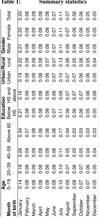
In addition to the standard publicly available information in the LFS, we also use the month-of-birth and year-of-birth information we can obtain from TURKSTAT.8Both month-of-birth and year-of-birth information in the survey come from interviewees’ own responses in a setting based on face-to-face interviewing. There is no cross-check from administrative and other official records to test the correctness of the responses. Table 1 documents the basic summary statistics for our sample. The total number of observations in our sample is 4,624,686. In the whole sample, the fraction of January-born individuals
8Note that this information is not publicly available. We thank the staff of the Labor Force Statistics Group in
is around 0.20. January-born individuals are evenly distributed across gender categories, while their fraction is higher among rural, older, and less-educated individuals. We also observe a rather smaller clustering for July. In Section 3, we provide a detailed explana-tion of the structural reasons why the density of people born in January and July is higher than those born in the other months.
3. Empirical analysis and discussion
In this section, we provide an empirical analysis of the season-of-birth patterns in Turkey. We proceed in four steps. First, we find that the month-of-birth distribution is strikingly asymmetric in Turkey. In particular, we report that, for a significant fraction of individ-uals in Turkey, the month of birth has been reported as January. We also show that this tendency is more pronounced for older cohorts. Second, we discuss the potential drivers of this asymmetry. Third, we investigate whether having January as the month of birth is correlated with educational outcomes, labor market outcomes, and the parental back-ground of the individuals. Finally, we present convincing evidence that the month-of-birth patterns in Turkey significantly reduce the reliability of certain quasi-experimental tech-niques – in particular, the regression discontinuity design – used to evaluate public policy, unless handled with caution.
3.1 Season-of-birth patterns in Turkey
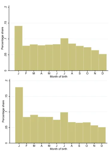
We start our analysis by providing a descriptive perspective for the season-of-birth pat-terns in Turkey. If the month of birth were totally random and there were no seasonality, then there should be an even distribution of individuals across the months, i.e., the month-of-birth probability should be 1/12≈0.083, for each month, for all individuals. But we provide strong evidence that there is no such symmetry in the month-of-birth patterns in Turkey. Specifically, we show that there is a strong tendency for having January as the birth month and that the incidence of being registered as January-born is higher for older cohorts.
Table 1: Summary statistics Ag e Education Urban/Rural Gender Month 0–19 20–39 40–59 Abo v e 60 Belo w HS and Urban rur al Male F emale T otal of bir th HS abo v e J an uar y 0.14 0.18 0.26 0.34 0.21 0.16 0.19 0.22 0.21 0.20 0.20 F ebr uar y 0.08 0.08 0.09 0.07 0.08 0.09 0.08 0.08 0.08 0.08 0.08 March 0.08 0.09 0.09 0.08 0.09 0.09 0.09 0.09 0.09 0.09 0.09 Apr il 0.08 0.08 0.08 0.06 0.08 0.08 0.08 0.08 0.08 0.08 0.08 Ma y 0.08 0.08 0.08 0.06 0.08 0.08 0.08 0.07 0.08 0.08 0.08 J une 0.08 0.08 0.06 0.06 0.07 0.08 0.07 0.07 0.07 0.07 0.07 J uly 0.10 0.10 0.11 0.17 0.11 0.09 0.10 0.13 0.11 0.11 0.11 A ugust 0.09 0.07 0.05 0.04 0.06 0.07 0.07 0.06 0.06 0.07 0.07 September 0.08 0.06 0.05 0.03 0.06 0.07 0.07 0.05 0.06 0.06 0.06 October 0.07 0.07 0.05 0.03 0.06 0.07 0.06 0.06 0.06 0.06 0.06 No v ember 0.07 0.06 0.04 0.03 0.05 0.06 0.06 0.05 0.05 0.05 0.05 December 0.05 0.05 0.04 0.03 0.05 0.06 0.05 0.04 0.05 0.05 0.05
Note: The table reports the distribution of the population across the months of birth with respect to the specified variable. 2004–2013 waves of the Turkish Household Labor Force Survey are used. The total number of observations in our sample is 4,624,686.
Figure 1: Month-of-birth distribution
0
.05
.1
.15
.2
Percentage share
J F M A M J J A S O N D
Month of birth
The sample contains individuals aged 0-19 from survey years 2004-2013
0
.05
.1
.15
.2
Percentage share
J F M A M J J A S O N D Month of birth
The sample contains individuals aged 20-39 from survey years 2004-2013
Note: The sample above contains individuals aged 0–19 from survey years 2004–2013. The sample below contains
individuals aged 20–39 from survey years 2004–2013.
registered as born in the other months; 2) the extent of this asymmetry is much larger for older cohorts than the younger cohorts; 3) July is another month we see clustering (much less than in January, however); and 4) it is almost invariably observed across age groups that the birth probabilities decline steadily over the year. In the next subsection, we discuss the potential factors that can explain these season-of-birth patterns and the associated asymmetries.9
9We should also mention at this point that in certain cases the existence of seasonality is not surprising, and
Figure 2: Month-of birth-distribution
0
.05
.1
.15
.2
.25
.3
.35
.4
Percentage share
J F M A M J J A S O N D
Month of birth
The sample contains individuals aged 40-59 from survey years 2004-2013
0
.05
.1
.15
.2
.25
.3
.35
.4
Percentage share
J F M A M J J A S O N D
Month of birth
The sample contains individuals above 60 from survey years 2004-2013
Note: The sample above contains individuals aged 40–59 from survey years 2004–2013. The sample below
con-tains individuals above 60 years of age from survey years 2004–2013.
3.2 Potential drivers of the season-of-birth patterns
The underlying force driving these asymmetries is the tendency to report the birth date in January – January 1 in particular. There are several factors that lead to misreporting. The first is related to the institutional setup, which is a combination of the regulations, geographical factors, and seasonal factors. The proportion of rural population is typically high in Turkey, and it was even higher in the past.10 Until the late 1980s, transportation,
health, and related infrastructure services were not highly developed in the rural regions of the country. The connections between city centers and villages were mostly broken during winter due to weather conditions.11 Anecdotal evidence suggests that, in some regions, the duration of the disconnect was around 6–7 months – i.e., from November to
10Around 20–25% of the population lives in rural areas based on the most recent figures. It was approximately
50% in the 1960s.
11This was a particular concern for the eastern and northern parts of the country, which are surrounded by high
April. Births in these regions during winter season were reported all at once to the Civil Registration Unit by the village headmen after the winter season. The convention was to report the date of birth as January 1 of the corresponding year. The birth registration system allowed for such flexibility in the past, while the current rules are strict and require official documentation of the date of birth issued by a hospital or health agency. As a result, the tendency to report January as the month of birth is due to a combination of institutional, geographical, and seasonal factors. The exact birth dates of the individuals in these category are mostly unknown.
The second mechanism is related to teenage marriages, which are currently rather rare in Turkey but were quite common in the past. Teenage marriages are mostly per-formed through religious ceremonies, since the laws do not permit legal marriages below age 18.12 Although teenage marriages are unlawful, they are mostly socially approved
since, in general, a religious ceremony is publicly held. Children born out of these mar-riages are not officially registered until their parents turn age 18. After age 18, parents get married legally and the children are officially registered. Their birth dates are very often recorded as January of the year after the parents get legally married. The two factors listed above account for a big chunk of the ‘January effect’ in birth records. The Anadolu Agency (the government-operated news agency in Turkey) documented that in January 2012, around 20% of the individuals residing in the Siverek province of Sanliurfa (a large city in southeastern Turkey) have January 1 as their birthday – 40,000 individuals out of a total of 200,000.
Third, another type of selection might also be operating in the background, which is not necessarily driven by the mechanisms explained above. This factor is related to parents’ perception about the school starting age of children. Specifically, some parents believe that children who start school early achieve worse educational outcomes relative to the ones who start late. There are also several empirical papers in the literature sup-porting the validity of this belief.13 Based on these concerns, parents of children who are
born later in a given year (i.e., in October, November, or December) may choose to report the birth month of their children as the January of the following year. As a consequence of this choice, the children will be among the oldest students in class, while they would be among the youngest had the parents reported correctly. There is some anecdotal evidence that this might also be a relevant mechanism. But it is definitely a minor factor relative to the other two factors outlined above. On a similar note, some parents may also tend to misreport to delay the compulsory military service for their male children.
These three factors explain the ‘January effect’ documented by Figures 1 and 2.
12More precisely, individuals can legally get married only if they have completed age 17.
13See, e.g., Bedard and Dhuey (2006), McEwan and Shapiro (2008), and Elder and Lubotsky (2009). We
Clearly, the tendency for misreporting has declined over time. There are three main reasons for this decline. First, the health system, transportation services, and the related infrastructure have significantly improved over time. Second, Turkey has seen several reforms to improve the accuracy of the civil registration system including a new census system as well as fully computerized population monitoring. And, third, enforcement has become more strict; there are now increased fines and other forms of punishment for misreporting the birth date or reporting the birth late. Although the misreporting tendency has significantly declined over time, the data suggests that it is still somewhat widespread in the new generation (see the upper panel of Figure 1).
There is also a smaller, but non-negligible, ‘July effect’ to be observed in the data. For all age groups, the probability of being July-born is significantly larger than the neu-tral probability of 0.083. To be precise, the fraction of individuals who are born in July is approximately 0.11, 0.10, 0.11, and 0.17 for age groups 0–19, 20–39, 40–59, and above 60, respectively. Again, the likelihood of being July-born is larger for older cohorts. Unlike the January effect, which was an artifact of misreporting, the July effect is more likely due to data imputation. There is a certain fraction of individuals (mostly old indi-viduals) for whom the month of birth is missing and only the year of birth is known. In some waves of the survey, interviewers entered July as the month of birth for those whose month of birth is missing. This is mainly performed for the purpose of approximating the age of the individual, which is a key variable in the data. We believe that this imputation is the main force driving the July effect.
The factors listed above are consistent with the observed patterns in the season of birth. These factors also suggest that certain types of individuals tend to misreport the birth dates of their children. These are most likely poor, uneducated individuals living in rural areas. That said, we cannot totally rule out the possibility that highly educated, well-off parents may also have incentives to misreport their children’s birth dates. For example, they may want to postpone the birth registration of their male children to delay military service. Similarly, they may misreport the birth dates for children to start schooling at an earlier or a later age. In the rest of the paper, we document that the season of birth variable is systematically correlated with educational outcomes of both the parents and children. We also demonstrate that these correlations can severely distort empirical policy evaluation exercises.
3.3 Education and labor market outcomes
outcomes. However, the outcomes may also differ with respect to season of birth due to selective seasonality in actual fertility behavior, as explained in Section 1. Unfortunately, the data does not allow us to clearly distinguish misreporting effects from the effects of actual fertility behavior.
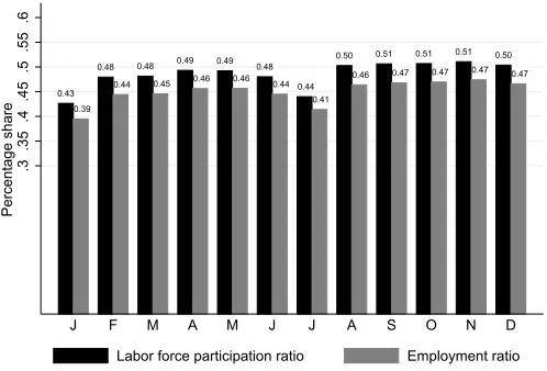
Figure 3 summarizes employment outcomes with respect to month of birth. We re-strict our sample to the individuals above age 30 for the purpose of concentrating on the ones who have completed their schooling. We focus on two outcomes: labor force par-ticipation ratio and the employment-to-population ratio. The figure suggests that both the employment-to-population ratio and the labor force participation ratio are approximately 5–6 percentage points lower in January than the average of the other months. In other words, the ones who have misreported birth dates are the ones who are less likely to be employed and who have low labor market attachment levels. Note that the July effect on employment outcomes is also significant yet less prominent than the January effect.
Figure 3: Labor force participation and employment across months of birth
0.43 0.39
0.48 0.44
0.48 0.45
0.49 0.46
0.49 0.46
0.48 0.44 0.44
0.41 0.50
0.46 0.51
0.47 0.51
0.47 0.51
0.47 0.50
0.47
.3
.35
.4
.45
.5
.55
.6
Percentage share
The sample contains individuals above 30 from all survey years 2004-2013
J F M A M J J A S O N D
Labor force participation ratio Employment ratio
Figure 4 documents the differences in real wages with respect to the month of birth. The nominal wages are deflated with the consumer price index (CPI), taking 2004 as the base year, to obtain real wages.
Figure 4: Real wages across months of birth
500
600
700
Real wage
J F M A M J J A S O N D
The sample contains salary employees from all survey years 2004-2013. The monthly wages were deflated to 2004 levels using consumer price index.
Note: The sample contains salaried employees from all survey years 2004–2013. The monthly wages were deflated
to 2004 levels using the consumer price index.
We observe a similar story with regard to real wages; that is, the real wages for those workers whose month of birth is reported as January earn around 10–12% less than those who were born early. While a July effect is also observed, it is not as strong as the January effect. One important observation regarding the month-of-birth effects on labor market outcomes is that the labor market outcomes for those who were born later in the year are better than for those who were born early. This pattern is not directly related to the January effect. In fact, there might also be seasonality in fertility behavior for the ones with better socioeconomic background – similar to what Buckles and Hungerman (2013) document. The data set we analyze, however, does not allow us to isolate the misreporting effect apart from the seasonality in the fertility behavior.
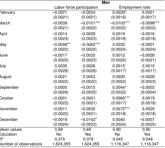
2, 4, 6, and 8 but excluded from others. We document that in the sample of men the difference in labor force participation probabilities between January-born individuals and individuals born in other months is not statistically significant. For the sample of women, we find that labor force participation probability is higher for those born in January even after controlling for education. There is no statistically significant gap between January-born men and others in terms of the employment-to-labor-force ratio. For the sample of women, the employment-to-labor-force ratio is higher among women born in January compared to other women.14This is not surprising, because the January-born individuals
are likely to have lower socioeconomic status, live in disadvantaged parts of the coun-try, and look for a job more desperately. Next, we further refine the analysis and look at the quality of employment in terms of wages and formal/informal employment across registered months of birth.
14In our own calculations, we find that the results are almost identical if we analyze the effect on
Table 2: Labor force participation and employment
Men
Labor force participation Employment ratio
February –0.0021 –0.0034 0.0029* 0.0001
(0.0021) (0.0021) (0.0016) (0.0017)
March –0.0039 –0.0101*** –0.0103*** –0.0098***
(0.0021) (0.0022) (0.0022) (0.0022)
April –0.0014 –0.0028 0.0019 –0.0016
(0.0023) (0.0023) (0.0018) (0.0018)
May –0.0048** –0.0062*** 0.0032 –0.0001
(0.0022) (0.0022) (0.0024) (0.0024)
June –0.0017 –0.0033 0.0012 –0.0026
(0.0022) (0.0023) (0.0020) (0.0021)
July 0.0035 0.0026 0.0015 0.0010
(0.0029) (0.0028) (0.0017) (0.0017)
August 0.0021 0.0003 0.0020 –0.0028
(0.0022) (0.0022) (0.0022) (0.0023)
September 0.0005 –0.0015 0.0044* –0.0003
(0.0029) (0.0025) (0.0022) (0.0024)
October –0.0001 –0.0021 0.0060*** 0.0019
(0.0022) (0.0021) (0.0017) (0.0018)
November –0.0011 –0.0032 0.0072*** 0.0025
(0.0022) (0.0021) (0.0018) (0.0018)
December –0.0019 –0.0142* 0.0040 –0.0007
(0.0024) (0.0023) (0.0024) (0.0025)
Mean values 0.69 0.69 0.90 0.90
Education No Yes No Yes
R2 0.374 0.379 0.045 0.049
Table 2: (Continued)
Women
Labor force participation Employment ratio
February –0.0041 –0.0115*** –0.0109*** –0.0105***
(0.0025) (0.0016) (0.0039) (0.0038)
March –0.0039 –0.0101*** –0.0103*** –0.0098***
(0.0029) (0.0019) (0.0037) (0.0035)
April –0.0008 –0.0091*** –0.0105** –0.0099**
(0.0032) (0.0021) (0.0045) (0.0043)
May –0.0044 –0.0118*** –0.0116*** –0.0109***
(0.0032) (0.0020) (0.0035) (0.0035)
June 0.0004 –0.0097*** –0.0118*** –0.0116***
(0.0032) (0.0024) (0.0042) (0.0041)
July 0.0017 0.0007 –0.0043 0.0047
(0.0048) (0.0036) (0.0056) (0.0055)
August 0.0020 –0.0131*** –0.0141*** –0.0137***
(0.0045) (0.0025) (0.0048) (0.0048)
September 0.0013 –0.0126*** –0.0100** –0.0091*
(0.0040) (0.0023) (0.0047) (0.0046)
October –0.0025 –0.0139*** –0.0129** –0.0126**
(0.0038) (0.0024) (0.0050) (0.0048)
November 0.0033 –0.0140*** –0.0159*** –0.0157***
(0.0036) (0.0026) (0.0034) (0.0032)
December –0.0018 –0.0153*** –0.0089** –0.0081*
(0.0051) (0.0031) (0.0042) (0.0040)
Mean values 0.25 0.25 0.88 0.88
Education No Yes No Yes
R2 0.145 0.202 0.089 0.093
Number of observations 1,751,367 1,751,367 442,385 442,385
Note: ***, **, and * refer to 1%, 5%, and 10% significance levels, respectively. First dependent variable is a binary
indicator that takes the value 1 if an individual is in the labor force, and 0 otherwise. The other dependent variable is a binary indicator for being employed conditional on labor force participation, and 0 otherwise. All individuals of age 15 and above from the 2004–2013 waves of the Turkish Household Labor Force Survey are included in the sample. Robust standard errors clustered at the regional (urban/rural) level are reported in parentheses (52 clusters in total). The coefficients should be read relative to January (the omitted month-of-birth dummy). The six education categories include no degree, primary school, middle school, high school, vocational high school, and college and above. Other controls include dummies for age, gender, marital status, urban/rural status, region, and survey year.
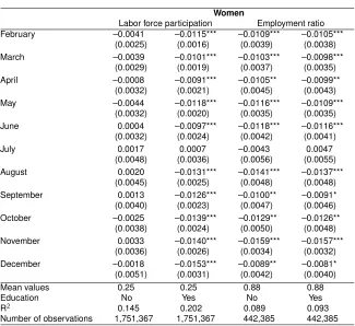
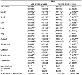
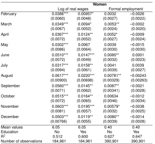
region dummies, and survey year dummies. We find that part of the January effect is not explained by education and other controls for real wages and formal/informal em-ployment. For real wages, the unexplained gap between January and other months is approximately 5% before controlling for education and it goes down to around 2% after including the education controls. This is in line with the findings in Table 4. January-born individuals have lower education levels on average, and this explains part of the wage gap between January-born individuals and those who were registered as born in other months. So, January-born individuals are likely to earn less even after controlling for the observed determinants of wages. The same is true for formal employment. On average, January-born individuals are less likely to be employed in formal jobs, and the gap is more evident in the sample of men. The results presented in Tables 2 and 3 complement each other. In terms of rough employment and labor force participation outcomes, there are no impor-tant differences between January-born individuals and others, especially in the sample of men.15However, the composition of employment differs substantially. The ones who are
registered as January-born are more likely to be employed in ‘bad’ jobs, i.e., low-paying and informal jobs.
Table 3: Real wages and formal employment
Men
Log of real wages Formal employment
February 0.0392*** 0.0172*** 0.0140*** 0.0077***
(0.0038) (0.0034) (0.0028) (0.0025)
March 0.0396*** 0.0190*** 0.0175*** 0.0118***
(0.0051) (0.0035) (0.0026) (0.0020)
April 0.0401*** 0.0152*** 0.0178*** 0.0106***
(0.0055) (0.0037) (0.0036) (0.0028)
May 0.0394*** 0.0153*** 0.0152*** 0.0085***
(0.0052) (0.0035) (0.0028) (0.0024)
June 0.0479*** 0.0190*** 0.0163*** 0.0088***
(0.0062) (0.0040) (0.0036) (0.0027)
July 0.0233*** 0.0136*** 0.0049 0.0037
(0.0075) (0.0040) (0.0036) (0.0029)
August 0.0596*** 0.0260*** 0.0215*** 0.0121***
(0.00648) (0.00403) (0.00315) (0.00223)
September 0.0633*** 0.0295*** 0.0218*** 0.0125***
(0.0062) (0.0038) (0.0040) (0.0030)
October 0.0567*** 0.0250*** 0.0200*** 0.0119***
(0.0077) (0.0051) (0.0041) (0.0032)
November 0.0647*** 0.0308*** 0.0244*** 0.0152***
(0.0081) (0.0056) (0.0040) (0.0031)
December 0.0627*** 0.0308*** 0.0205*** 0.0112**
(0.0070) (0.0039) (0.0053) (0.0043)
Mean values 6.17 6.17 0.62 0.62
Education No Yes No Yes
R2 0.443 0.528 0.369 0.379
Table 3: (Continued)
Women
Log of real wages Formal employment
February 0.0386*** 0.00957* 0.0032 –0.0026
(0.0060) (0.0048) (0.0027) (0.0022)
March 0.0349*** 0.0094* 0.0053** –0.0002
(0.0067) (0.0052) (0.0024) (0.0020)
April 0.0367*** 0.0124** 0.0052* –0.0009
(0.0072) (0.0052) (0.0027) (0.0024)
May 0.0302*** 0.0067 0.0039 –0.0015
(0.0086) (0.0064) (0.0030) (0.0030)
June 0.0510*** 0.0147*** 0.0080** 0.0001
(0.0072) (0.0049) (0.0032) (0.0023)
July 0.0317*** 0.0158** 0.0041 0.0039
(0.0094) (0.0061) (0.0039) (0.0027)
August 0.0617*** 0.0220*** 0.00781** –0.00243
(0.00900) (0.00698) (0.00329) (0.00263)
September 0.0560*** 0.0145** 0.0087** –0.0021
(0.0071) (0.0062) (0.00341) (0.0028)
October 0.0515*** 0.0164** 0.00634 –0.0012
(0.0072) (0.0065) (0.0046) (0.0034)
November 0.0603*** 0.0195*** 0.00579* –0.0038
(0.0081) (0.0057) (0.0032) (0.0025)
December 0.0503*** 0.0119** 0.0080** –0.0014
(0.00766) (0.0055) (0.0039) (0.0028)
Mean values 6.05 6.05 0.40 0.40
Education No Yes No Yes
R2 0.512 0.600 0.627 0.647
Number of observations 184,961 184,961 390,901 390,901
Note:***, **, and * refer to 1%, 5%, and 10% significance levels, respectively. First dependent variable is log of real
Figures 5–7 reveal that there are huge differences between months of birth with respect to educational outcomes. Figure 5 plots the high school and college graduation rates.16 Clearly, there is a huge January effect for both outcomes. To be specific, the high school and college graduation rates for January-born adults are 0.15 and 0.6, respectively, while these rates are 0.31 and 0.13, respectively, for an average October-born adult. We also observe that there is a significant July effect in educational outcomes; that is, the high school and college graduation rates for an average July-born individual are 0.16 and 0.07, respectively.
Figure 5: Educational attainment across months of birth
0.15
0.06 0.24
0.10 0.23
0.10 0.25
0.10 0.25
0.10 0.25
0.11 0.16
0.07 0.30
0.13 0.31
0.13 0.28
0.12 0.30
0.13 0.29
0.13
0
.05
.1
.15
.2
.25
.3
.35
Percentage share
The sample contains individuals above 30 from all survey years 2004-2013
J F M A M J J A S O N D
High school and above Two-year college and above
Note: The sample above contains individuals above age 30 from all survey years 2004–2013.
16High school graduates include those who have a high school degree or a higher one. College graduates
Figures 6 and 7 show that these strong month-of-birth effects in education hold in-variably across different birth cohorts and also across gender categories.
We also check whether observed education levels vary across months of birth. Ta-ble 4 reports the regression results. We focus on three outcomes: years of completed schooling (column 1), high school graduation and above (column 2), and college gradua-tion (column 3). The control variables include gender, age, marital status, an urban/rural indicator, region dummies, and survey year dummies. We find that the observed vari-ables such as gender, age, and region of residence can explain only a small fraction of the raw January effect in education outcomes. To be concrete, we find that, on average, the January-born individuals stop schooling approximately 0.6 years early and that they are around 7 percentage points less likely to complete high school education or above.
Figure 6: High school completion rates across months of birth, by gender
0
.1
.2
.3
.4
.5
.6
High school completion ratio
J-71 J-72 J-73 J-74 J-7 J-76 J-77 J-78 J-79 J-80 Month of birth
Men Women
The sample contains individuals from survey years 2004-2013 who were born in 1971-1980. The vertical axis shows the ratio of those with high school degree and above.
Those who were born in January are gridded.
Note: The sample contains individuals from survey years 2004–2013 who were born between 1971 and 1980. The
Figure 7: College completion rates across months of birth, by gender
0
.1
.2
.3
College degree ratio
J-71 J-72 J-73 J-74 J-7 J-76 J-77 J-78 J-79 J-80 Month of birth
Men Women
The sample contains individuals from survey years 2004-2013 who were born in 1971-1980. The vertical axis shows the ratio of those with 2-year college degree and above. Those who were born in January are gridded.
Note: The sample contains individuals from survey years 2004–2013 who were born between 1971 and 1980. The
Table 4: Registered month of birth and educational outcomes
Men Women
Years of s. H.s. ratio College ratio Years of s. H.s. ratio College ratio
January omitted omitted omitted omitted omitted omitted
(0.059) (0.007) (0.004) (0.052) (0.006) (0.003)
March 0.515*** 0.061*** 0.035*** 0.353*** 0.041*** 0.017***
(0.065) (0.008) (0.005) (0.060) (0.007) (0.003)
April 0.603*** 0.071*** 0.038*** 0.429*** 0.050*** 0.022***
(0.065) (0.008) (0.005) (0.067) (0.008) (0.004)
May 0.579*** 0.067*** 0.040*** 0.413*** 0.049*** 0.019***
(0.068) (0.008) (0.005) (0.070) (0.009) (0.004)
June 0.679*** 0.079*** 0.047*** 0.472*** 0.056*** 0.024***
(0.097) (0.011) (0.007) (0.083) (0.010) (0.004)
July 0.095 0.011 0.007 0.081 0.009 0.003
(0.104) (0.012) (0.008) (0.097) (0.011) (0.006)
August 0.926*** 0.109*** 0.061*** 0.674*** 0.079*** 0.036***
(0.106) (0.012) (0.008) (0.092) (0.011) (0.005)
September 0.956*** 0.111*** 0.065*** 0.719*** 0.083*** 0.037***
(0.107) (0.013) (0.008) (0.099) (0.012) (0.057)
October 0.750*** 0.087*** 0.053*** 0.546*** 0.063*** 0.028***
(0.088) (0.011) (0.007) (0.084) (0.010) (0.005)
November 0.867*** 0.099*** 0.061*** 0.668*** 0.078*** 0.037***
(0.106) (0.013) (0.008) (0.095) (0.012) (0.005)
December 0.848*** 0.097*** 0.057*** 0.672*** 0.077*** 0.033***
(0.096) (0.012) (0.007) (0.0100) (0.011) (0.006)
Mean value 7.53 0.29 0.12 6.36 0.16 0.06
Controls Yes Yes Yes Yes Yes Yes
R2 0.131 0.114 0.052 0.161 0.140 0.075
3.4 Parental background
Next we focus on the relationship between one’s month of birth and parental background. For this purpose, we focus on children of below age 15. Figures 8 and 9 summarize the differences in maternal and paternal education in terms of month of birth. Although the incidence of misreporting appears to diminish for younger individuals, we still observe a systematic relationship between being January-born and having parents with worse ed-ucational backgrounds. We see that this tendency holds for both maternal and paternal education. Specifically, we find that the mothers of January-born children have, on av-erage, 0.3 years less completed education than the mothers of children born in the other months. The magnitude for the paternal education gap is slightly higher at around 0.35 years on average.
Figure 8: Mother’s years of education across months of birth
6.19 6.34 6.38 6.45 6.55 6.54 6.46 6.50 6.52 6.49 6.50 6.36
5
6
7
8
Years of education
J F M A M J J A S O N D
The sample contains mothers of children below 15 from all survey years 2004-2013 The horizontal axis shows the registered months of birth of children.
Note: The sample contains mothers of children under age 15 from survey years 2004–2013. The horizontal axis
Figure 9: Father’s years of education across months of birth
7.23 7.47 7.48 7.56
7.66 7.68 7.58 7.64 7.63 7.63 7.65 7.47
5
6
7
8
Years of education
J F M A M J J A S O N D
The sample contains fathers of children below 15 from all survey years 2004-2013. The horizontal axis shows the registered months of birth of children.
Note: The sample contains fathers of children under age 15 from survey years 2004–2013. The horizontal axis
shows the registered months of birth of children.
Table 5: Parental education and registered month of birth (dependent variable: being born in January)
Men Women
Mother’s years of education –0.0009*** –0.0005 (0.0003) (0.0003) Father’s years of education –0.0013*** 0.0015***
(0.0003) (0.0003)
Urban –0.0145*** –0.0123
(0.0022) (0.0028)
Mean value 0.1364 0.1319
Controls Yes Yes
R2 0.020 0.019
Number of observations 583,983 556,787
Note:***, **, and * refer to 1%, 5%, and 10% significance levels, respectively. The dependent variable is a binary
indicator that takes the value 1 if registered month of birth is January and 0 otherwise. All individuals below age 15 from the 2004–2013 waves of the Turkish Household Labor Force Survey are included in the sample. Robust standard errors clustered at the regional (urban/rural) level are reported in parentheses (52 clusters in total). The coefficients should be read relative to January (the omitted month-of-birth dummy). Other controls include dummies for year of birth, gender, marital status, urban/rural status, region, and survey year.
3.5 Implications for policy evaluation
Quasi-experimental designs have become increasingly popular tools used by economists in evaluating the effectiveness of public policies. An unexpected exogenous change in the economic environment is the main requirement of a quasi-experimental design. Most of the time, such an unexpected change comes from a policy reform. For some reforms, there is a sharp cutoff date describing eligibility. There are several examples for such policy reforms in Turkey. For example, the 1997 education reform extended the compul-sory schooling from 5 years to 8 years. The eligibility is implicitly defined in terms of the date of birth. Specifically, the ones who were born in or after 1987 were forced to continue education until the eighth grade, while those who were born before 1987 were not.17Another example is the 1999 compulsory military service (paid) exemption reform.
The ones who were born on or before December 31, 1972, were eligible for the paid ex-emption, while those who were born on or after January 1, 1973, were not eligible.18 In an ideal setting, a regression discontinuity design (RDD) will identify the impact of the reform. The prerequisite for having an ‘ideal setting’ in an RDD is that the reform should resemble a randomized experiment in such a way that the cutoff date randomly separates the ones who benefit from the ones who do not.
17See Aydemir and Kirdar (2017) and Torun (2015) for the details of the reform.
18See Torun and Tumen (2016) for the causal impact of this reform on educational and labor market outcomes
To be more concrete, suppose that we have a policy reform at hand that separates the treatment group from the control group based on the birth dates of the subjects. Suppose further that, just as with the compulsory military service exemption reform mentioned above, the ones who were born on or before December 31, 1972, are in the treatment group, while those who were born on or after January 1, 1973, are placed into the control group. As stated in Torun and Tumen (2016), the ones who were born before the cutoff date were allowed to be exempt from military service by paying a certain amount of money, while the ones who were born after the cutoff date were not given that option. The effect of being exposed to compulsory military service early in life on later outcomes is the subject of an ongoing debate in the literature. Angrist (1990) and Imbens and van der Klaauw (1995) find that those who served in the army earn fewer wages after their service. On the other hand, Grenet, Hart, and Roberts (2011), Bauer et al. (2012), and Paloyo (2010) find no effect of conscription on future earnings. There are also studies that examine the effect of conscription on health and crime (Angrist, Chen, and Frandsen 2010; Bedard and Deschenes 2006; Galiani, Rossi, and Schargrodsky 2011). The paid exemption policy provides an opportunity to compare the outcomes of the ones who are exempt to those of the ones who are not. Based on this definition, the ones who are born before the cutoff (and, thus, allowed to be exempt) are designated as ‘treated,’ while the ones who are born after the cutoff date are designated as ‘control.’ The main problem here is that, although the policy reform constitutes an unexpected and exogenous change in the economic environment, the distribution of individuals around the reform date prevents the formation of an artificial randomization. The evidence we provide above suggests that the January-born individuals are systematically different from the December-born individuals in the sense that, on average, they have worse educational and labor market outcomes. Moreover, their parents have worse socioeconomic characteristics. In such a setup, whether there is an actual treatment or not, we expect to see that the outcomes of the January-born individuals should be worse than the outcomes of the December-born individuals for any birth year.
To confirm the validity of this conjecture, we perform RDD exercises for the purpose of comparing the real earnings of individuals born right before and after January 1, just as if January 1 were the reform cutoff date. We execute this exercise for ten different birth cohorts, from 1965 to 1975. We set a two-month window, from December in year tto January in yeart+ 1. The observations for December in yeartrepresent the treated outcomes, while the observations for January in yeart+1represent the control outcomes. Note that, unlike in the United States, the compulsory schooling laws in Turkey do not have age cutoffs – i.e., children in the United States are required to be enrolled in school until their 15th or 16th birthdays (depending on the state of residence) while in Turkey
different outcomes. Each of these exercises is performed based on the placebo assumption that there is a policy reform putting the December-born individuals in year t into the treatment group and the January-born individuals in yeart+ 1into the control group. We basically compare the outcomes of December-born individuals to those of the January-born ones. The outcomes of interest are the monthly labor market earnings (including performance pay, bonuses, etc.) and the years of completed education. The covariates include gender, age dummies, urban/rural dummies, region dummies, and survey year dummies. The first two columns report the results of the earnings regressions. column 1 excludes the education dummies, while column 2 includes them as control variables.19
Column 1 suggests that for almost all birth year cohorts, the treatment outcome is positive and statistically significant. In other words, for each exercise, we find a positive effect of being born in December as if there were an actual policy reform. The magnitude of the effect on earnings is around 11% on average. Based on the discussion presented above, we conclude that this result should be fully attributed to the January effect. Column 2 suggests that the effect disappears in most samples when we control for education. As the results of a complementary exercise, column 3 suggests that the January effect on earnings is driven by the January effect on education. This result is consistent with the results presented in Sections 3.3 and 3.4.20
19Note that the standard errors in the RDD exercises are clustered at the geographical level to maintain
consis-tency with the previous regressions, although it would be more natural to cluster at the month level since ‘month’ is the running variable in our RDD exercises. The main reason for this choice is that the number of clusters will be very small at the month level, which pushes standard errors down and makes all the coefficients strongly significant. Both for being conservative and maintaining the consistency of the empirical setup throughout the paper, we chose to cluster the standard errors at the geographical level also for the RDD exercises.
20It would be useful to clarify how the coefficients displayed in the regression tables should be interpreted. In
Table 6: Regression discontinuity design
Log earnings Years of education
1 2 3
Treatment (1965–1966) 0.1730*** 0.0351 1.0027***
(0.0308) (0.0219) (0.1560)
Treatment (1966–1967) 0.0896** –0.0024 0.9150***
(0.0339) (0.0220) (0.1510)
Treatment (1967–1968) 0.0918*** 0.0113 0.7970***
(0.0329) (0.0248) (0.0169)
Treatment (1968–1969) 0.1580*** –0.0017 0.9690***
(0.0355) (0.0199) (0.1560)
Treatment (1969–1970) 0.1200*** 0.0275 0.7410***
(0.0412) (0.0230) (0.1510)
Treatment (1970–1971) 0.1060*** 0.0268 0.7620***
(0.0291) (0.0193) (0.1380)
Treatment (1971–1972) 0.1380*** –0.0039 0.9310***
(0.0293) (0.0208) (0.1490)
Treatment (1972–1973) 0.0774*** –0.0143 0.8931***
(0.0274) (0.0217) (0.0847)
Treatment (1973–1974) 0.1150*** 0.0315 0.7759***
(0.0282) (0.0239) (0.1254)
Treatment (1974–1975) 0.1188*** 0.0328 0.9284***
(0.0282) (0.0223) (0.1405)
Education No Yes No
Other controls Yes Yes Yes
Note:***, **, and * refer to 1%, 5%, and 10% significance levels, respectively. First dependent variable is log of real
4. Concluding remarks
The season of birth is often used in labor economics as an instrumental variable (com-bined with compulsory schooling laws) that generates exogenous variation in years of completed education. The main assumption is that the month of birth is exogenous; that is, it cannot be manipulated or it is not systematically correlated with socioeconomic background and later outcomes. However, a large set of papers shows that there exists a systematic relationship between the season of birth and later outcomes (labor market outcomes, education, health, etc.). Explanations for this association mainly focus on fac-tors that generate seasonality in fertility behavior or seasonal exposure to nutrition and/or disease. These factors are employed in statistical analysis to provide evidence that season of birth has a behavioral component and that this component has further implications, which are non-negligible.
In this paper, we use a large micro-level data set from Turkey to show that a combi-nation of geographical, seasonal, and institutional factors can lead to a strong systematic association between registered season of birth and later outcomes. In particular, we show that there is a strong tendency to be registered as January-born in Turkey and that this ten-dency is higher for people with worse socioeconomic backgrounds, whose place of birth is mostly in rural areas. As a result, on average, there is a marked difference between the later outcomes of individuals who are born in December of yeart and those who were born in January of yeart+ 1. We also argue that these differences may lead to prob-lems that contaminate policy evaluation exercises relying on sharp discontinuities (such as regression discontinuity designs and IV) determined by cutoff birth dates. Examples of these policies include compulsory schooling and compulsory military service laws in Turkey, which set January 1 as the cutoff birth date.
References
Almond, D. (2006). Is the 1918 influenza pandemic is over? Long-term effects of in utero influenza exposure in the post-1940 US population.Journal of Political Economy 114(4): 672–712.doi:10.1086/507154.
Angrist, J.D. (1990). Lifetime earnings and the vietnam era draft lottery: Evidence from social security administrative records.American Economic Review80(3): 313–336.
Angrist, J.D., Chen, S.H., and Frandsen, B.R. (2010). Did Vietnam veterans get sicker in the 1990s? The complicated effects of military service on self-reported health.Journal of Public Economics94(11–12): 824–837. doi:10.1016/j.jpubeco.2010.06.001.
Angrist, J.D. and Krueger, A.B. (1991). Does compulsory schooling attendance ef-fect schooling and earnings? Quarterly Journal of Economics 106(4): 976–1014.
doi:10.2307/2937954.
Angrist, J.D. and Krueger, A.B. (1992). The effect of age at school entry on edu-cational attainment: An application on instrumental variables with moments from two samples. Journal of the American Statistical Association 87(418): 328–336.
doi:10.1080/01621459.1992.10475212.
Angrist, J.D. and Krueger, A.B. (1995). Split sample instrumental variables estimates for the return to schooling.Journal of Business and Economic Statistics13(2): 225–235.
Angrist, J.D. and Krueger, A.B. (2001). Instrumental variables and the search for iden-tification: From supply and demand to natural experiments. Journal of Economic Perspectives15(4): 69–85. doi:10.1257/jep.15.4.69.
Aydemir, A. and Kirdar, M.G. (2017). Low wage returns to schooling in a developing country: Evidence from a major policy reform in Turkey. Bonn: IZA Institute of Labor Economics (IZA discussion paper 9274).
Barker, D. (2001). Fetal and infant origins of adult disease. Monatsschrift f¨ur Kinder-heilkunde149(Supplement 1): 2–6.doi:10.1007/s001120170002.
Bauer, T.K., Bender, S., Paloyo, A.R., and Schmidt, C.M. (2012). Evaluating the labor-market effects of compulsory military service.European Economic Review56(4): 814– 829. doi:10.1016/j.euroecorev.2012.02.002.
Bedard, K. and Deschenes, O. (2006). The long-term impact of military service on health: Evidence from World War II and Korean war veterans. American Economic Review 96(1): 176–194. doi:10.1257/000282806776157731.
1437–1472.doi:10.1093/qje/121.4.1437.
Bjornsson, D.F. and Zoega, G. (forthcoming). Seasonality of birth rates in agricultural Iceland. Scandinavian Economic History Review
doi:10.1080/03585522.2017.1340333.
Bound, J. and Jaeger, D.A. (2001). Do compulsory school attendance laws alone ex-plain the association between quarter of birth and earnings? In: Bound, J. and Jaeger, D.A. (eds.).Research in labor economics. Bingley: Emerald Group: 83–108.
doi:10.1016/S0147-9121(00)19005-3.
Bound, J., Jaeger, D.A., and Baker, R.M. (1995). Problems with instrumental variables es-timation when the correlation between the instruments and the endogenous explanatory variable is weak. Journal of the American Statistical Association90(430): 443–450.
doi:10.1080/01621459.1995.10476536.
Buckles, K.S. and Hungerman, D.M. (2013). Season of birth and later outcomes: Old questions, new answers. Review of Economics and Statistics 95(3): 711–724.
doi:10.1162/REST a 00314.
Card, D. (1999). The causal effect of education on earnings. In: Bound, J. and Jaeger, D.A. (eds.).Handbook of labor economics. New York: Elsevier: 1801–1863.
doi:10.2307/2523702.
Cascio, E. and Lewis, E. (2006). Schooling and the armed forces qualifying test.Journal of Human Resources41(2): 294–318.doi:10.3368/jhr.XLI.2.294.
Cesur, R. and Mocan, N. (forthcoming). Education, religion, and voter preference in a Muslim country.Journal of Population Economicsdoi:10.1007/s00148-017-0650-3.
Dickert-Conlin, S. and Chandra, A. (1999). Taxes and the timing of births. Journal of Political Economy107(1): 161–177.doi:10.1086/250054.
Dobkin, C. and Ferreira, F. (2010). Do school entry laws affect educational attain-ment and labor market outcomes? Economics of Education Review 29(1): 40–54.
doi:10.1016/j.econedurev.2009.04.003.
Doblhammer, G., Scholz, R., and Maier, H. (2005). Month of birth and survival to age 105+: Evidence from the age validation study of German semi-supercentenarians. Ex-perimental Gerontology40(10): 829–835.doi:10.1016/j.exger.2005.07.012.
Dor´elien, A.M. (2016). Birth seasonality in sub-Saharan Africa.Demographic Research 34(27): 761–796.doi:10.4054/DemRes.2016.34.27.
Galiani, S., Rossi, M.A., and Schargrodsky, E. (2011). Conscription and crime: Evidence from the Argentine draft lottery. American Economic Journal: Applied Economics 3(2): 119–136.doi:10.1257/app.3.2.119.
Gans, J.S. and Leigh, A. (2009). Born on the first of July: An unnatural ex-periment in birth timing. Journal of Public Economics 93(1–2): 246–263.
doi:10.1016/j.jpubeco.2008.07.004.
Gelbach, J. (2002). Public schooling for young children and maternal labor supply. Amer-ican Economic Review92(1): 307–322. doi:10.1257/000282802760015748.
Gortmaker, S., Kagan, J., Caspi, A., and Silva, P. (1997). Daylength during pregnancy and shyness of children: Results from Northern and Southern hemi-sphere. Developmental Psychobiology 31(2): 107–114. doi:10.1002/(SICI)1098-2302(199709)31:2¡107::AID-DEV3¿3.0.CO;2-O.
Grenet, J., Hart, R.A., and Roberts, J.E. (2011). Above and beyond the call: Long-term real earnings effects of British male military conscription in the post-war years.Labour Economics18(2): 194–204. doi:10.1016/j.labeco.2010.09.001.
Hansen, K.T., Heckman, J.J., and Mullen, K. (2004). The effect of schooling and ability on achievement test scores. Journal of Econometrics 121(1–2): 39–98.
doi:10.1016/j.jeconom.2003.10.011.
Hoogerheide, L., Kleibergen, F., and van Dijk, H. (2007). Natural conjugate priors for the instrumental variables regression model applied to the Angrist–Krueger data. Journal of Econometrics138(1): 63–103. doi:10.1016/j.jeconom.2006.05.015.
Imbens, G.W. and van der Klaauw, W. (1995). Evaluating the cost of conscription in The Netherlands. Journal of Business and Economic Statistics 13(2): 207–215.
doi:10.1080/07350015.1995.10524595.
Knodel, J. and Wilson, C. (1981). The secular increase in fecundity in German village populations: An analysis of reproductive histories of couples married 1750–1899. Pop-ulation Studies35(1): 53–84. doi:10.2307/2174835.
LaLumia, S., Sallee, J.M., and Turner, N. (2015). New evidence on taxes and the timing of birth. American Economic Journal: Economic Policy 7(2): 258–293.
doi:10.1257/pol.20130243.
Lam, D.A. and Miron, J.A. (1994). Global patterns of seasonal variation in human fer-tility. Annals of the New York Academy of Sciences709: 9–28. doi:10.1111/j.1749-6632.1994.tb30385.x.
doi:10.1016/j.econedurev.2009.03.004.
Lefgren, L. and McIntyre, F. (2006). The relationship between women’s edu-cation and marriage outcomes. Journal of Labor Economics 24(4): 787–830.
doi:10.1086/506486.
Leigh, A. and Ryan, C. (2008). Estimating returns to education using different natural experiment techniques. Economics of Education Review 27(2): 149–160.
doi:10.1016/j.econedurev.2006.09.004.
Levin, J. and Plug, E. (1999). Instrument education and the returns to schooling in The Netherlands. Labour Economics6(4): 521–534. doi:10.1016/S0927-5371(99)00033-0.
Levy, V. (1986). Seasonal fertility cycles in rural Egypt: Behavioral and biological link-ages. Demography23(1): 13–30. doi:10.2307/2061405.
Livingston, R., Adam, B., and Bracha, H.S. (1993). Season of birth and neurodevelop-mental disorders: Summer birth is associated with dyslexia. American Academy of Child and Adolescent Psychiatry32(3): 612–616. doi:10.1097/00004583-199305000-00018.
Massey, D.S. and Mullan, B.P. (1984). A demonstration of the effect of seasonal migra-tion on fertility. Demography21(4): 501–517. doi:10.2307/2060912.
Maurin, E. and Moschion, J. (2009). The social multiplier and labor market participa-tion of mothers. American Economic Journal: Applied Economics1(1): 251–272.
doi:10.1257/app.1.1.251.
McEwan, P.J. and Shapiro, J.S. (2008). The benefits of delayed primary school enroll-ment: Discontinuity estimates using exact birth dates. Journal of Human Resources 43(1): 1–29.doi:10.3368/jhr.43.1.1.
Neugart, M. and Ohlsson, H. (2013). Economic incentives and the timing of births: Evidence from the German Parental Benefit Reform of 2007. Journal of Population Economics26(1): 87–108.doi:10.1007/s00148-012-0420-1.
Paloyo, A.R. (2010). Compulsory military service in Germany revisited. Essen: Leibniz-Institute for Economic Research (Ruhr Economic paper 206).
Plug, E. (2001). Season of birth, schooling, and earnings.Journal of Economic Psychol-ogy22(5): 641–660. doi:10.1016/S0167-4870(01)00060-5.
Robertsen, E. (2011). The effects of quarter of birth on academic outcomes at the elementary school level. Economics of Education Review 30(2): 300–311.
Schultz-Nielsen, M.L., Tekin, E., and Greve, J. (2016). Labor market effects of in-trauterine exposure to nutritional deficiency: Evidence from administrative data on Muslim immigrants in Denmark. Economics and Human Biology 21: 196–209.
doi:10.1016/j.ehb.2016.02.002.
Sham, P., O’Callaghan, E., Takei, N., Murray, G., Har, E., and Murray, R. (1992). Schizophrenia following pre-natal exposure to influenza epidemics between 1939 and 1960.British Journal of Psychiatry160(4): 461–466.doi:10.1192/bjp.160.4.461.
Skirbekk, V., Kohler, H.P., and Prskawetz, A. (2004). Birth month, school grad-uation, and the timing of births and marriages. Demography 41(3): 547–568.
doi:10.1353/dem.2004.0028.
Tochigi, M., Okazaki, Y., Kato, N., and Sasaki, T. (2004). What causes sea-sonality of birth in schizophrenia? Neuroscience Research 48(1): 1–11.
doi:10.1016/j.neures.2003.09.002.
Torun, H. (2015). Compulsory schooling laws and early labor market outcomes in a middle-income country. Ankara: Central Bank of the Republic of Turkey (Working paper 15/34).