DEMOGRAPHIC RESEARCH
VOLUME 35, ARTICLE 28, PAGES 813
−
866
PUBLISHED 22 SEPTEMBER 2016
http://www.demographic-research.org/Volumes/Vol35/28/ DOI: 10.4054/DemRes.2016.35.28
Research Article
GDP and life expectancy in Italy and Spain over
the long run: A time-series approach
Emanuele Felice
Josep Pujol Andreu
Carlo D’Ippoliti
©2016 Emanuele Felice, Josep Pujol Andreu & Carlo D’Ippoliti.
This open-access work is published under the terms of the Creative Commons Attribution NonCommercial License 2.0 Germany, which permits use, reproduction & distribution in any medium for non-commercial purposes, provided the original author(s) and source are given credit.
1 Introduction 814
2 How close, how far? A comparison by pairs of indicators
(1861–2008) 817
3 Trends in GDP and life expectancy 824
4 Time series analysis 827
4.1 Granger causality 827
4.2 Structural breaks and sub-period Granger causality 831
5 Conclusions 836
6 Acknowledgments 837
References 838
GDP and life expectancy in Italy and Spain over the long run:
A time-series approach
Emanuele Felice1
Josep Pujol Andreu2
Carlo D’Ippoliti3
Abstract
BACKGROUND
A growing body of literature focuses on the relationship between life expectancy and GDP per capita. However, available studies to date are overwhelmingly based on either cross-country or cross-sectional data. We address the issue from a novel, more historically grounded approach, i.e., comparing long-run consistent time series.
OBJECTIVE
To investigate what, if any, is the causal link between life expectancy and GDP. METHODS
We provide consistent and updated long-term yearly time series of GDP and life expectancy for Italy and Spain and compare them with those available for France. RESULTS
Both Italy and Spain converged towards the European core (France) earlier in life expectancy than in GDP. We find it necessary to split the series into two sub-periods, and we find that, in general, both improvements in life expectancy cause GDP growth and economic growth causes improvements in life expectancy. For the countries and the periods considered there are, however, exceptions in both cases.
CONCLUSIONS
Our findings confirm the hypothesis of a non-monotonic relationship between life expectancy and income, but they also emphasize the importance of empirical qualifications, imposed by the historical experience of each national case.
1. Introduction
There is a growing literature on the relation between improvements in life expectancy and the rise in gross domestic product (GDP) per capita. The subject is of the utmost interest to economists, demographers, and policymakers (at least in the developed countries, which are experiencing an ageing population and sluggish economic growth). A well-established causal link goes from income to life expectancy. According to Preston (1975), the relationship between GDP and life expectancy in the 20th century
follows a logarithmic curve. The impact of GDP on life expectancy is higher when the former is low, then it decreases as GDP rises, and even disappears after GDP reaches a certain threshold. While this relationship is widely accepted in the literature4 there is no
consensus on the opposite causal link, going from life expectancy to income.
In economics, the unified growth theory holds that the demographic transition plays a crucial role in initiating the shift from stagnation to growth (Galor and Weil 2000; Galor 2012): The idea is that with the demographic transition, higher life expectancy leads to lower fertility and lower population growth, and thus to higher returns of human capital investments to those living longer. In turn, lower fertility and higher human capital both contribute to the rise of per capita GDP. A number of cross-country studies find a positive effect of life expectancy, or a negative effect of mortality, on income per capita (Bloom and Sachs 1998; Gallup, Sachs, and Mellinger 1999; Lorentzen, McMillan, and Wacziarg 2008), but the debate is still ongoing. For example, Acemoglu and Johnson (2007) find no impact of life expectancy on GDP per capita, and their explanation is that increased life expectancy actually accelerates population growth. More recent studies suggest that the causal effect of life expectancy on growth is non-monotonic, i.e., it is negative but insignificant before the onset of the demographic transition, and positive afterwards (Cervellati and Sunde 2011).
All these studies are based on cross-sectional comparisons. By contrast, here we aim to exploit new and updated time series in order to investigate the issue from a historical perspective. We use updated long-run estimates of life expectancy and GDP for Italy and Spain (1861‒2008) and compare them with the available corresponding series for France. Indeed, the development and employment of these long series − an
approach that can be regarded as complementary to cross-sectional comparisons − is in itself one of the main contributions of our work. In macroeconomic history, two approaches are the most popular on quantitative grounds: cross-country studies, often
using cross-sectional data, and country-specific studies, usually employing time series. In cross-country studies the data at hand is typically limited to a few benchmark years or to short periods of time. Although a wide range of countries and indicators may be included and discussed, the lack of time series may prevent these studies from dealing efficaciously with endogeneity, even when instrumental variables are introduced, while heterogeneity or even inconsistency of the data used may be overlooked. Time-series macroeconomic analyses of specific countries or regions are of course much more complete in historical coverage and at times take advantage of refined estimates,5 but
this may be detrimental to international comparisons.6 A combination of the two
methods has also been used for international comparisons7 and in specific country
studies. For instance, limited to the Spanish case, Pérez Moreda, Reher, and Sanz Gimeno (2015: 292–299) compare GDP per capita and life expectancy/mortality in the long run by making use of both yearly series (at the national level, from 1901 to 1990) and cross-sectional data (at the regional level, in four benchmarks corresponding to the 1860s, 1900‒1901, 1930‒1931, and 1961), even though they only estimate simple correlations between the variables.
Here, we extend the time-series analysis to a comparison between countries, with a historical coverage spanning 148 years (1861–2008), and we also investigate the causal relationship between the two variables.8 We consider the two largest countries of
Southern Europe, Italy and Spain − which are usually regarded as similar in culture and
values, as well as with respect to some key institutional features and economic patterns9
− and compare them with France, their principal neighbour, the country that both have
often looked up to as providing proper terms of evaluation. These are big countries,
5 For Italy, see Fenoaltea (2003, 2005) and, more recently, Felice and Vecchi (2015a, 2015b). For Spain, see, among others, Pons and Tirado (2006), Prados de la Escosura and Rosés (2009), Prados de la Escosura (2010a), Sabaté, Fillat, and Gracia (2011) and Prados de la Escosura, Rosés, and Sanz-Villarroya (2012). For other countries, see, for instance, the remarkable study on Turkey by Altug, Filiztekin, and Pamuk (2008), or the recent reconstruction of Venezuelan GDP, 1830‒2012, by De Corso (2013).
6 Unless of course Maddison’s (2010) renowned series are used. However, when it comes to a detailed scrutiny of national cases, Maddison’s estimates are not always trustworthy and, above all, comparisons not always reliable (Felice 2016). For a critique of Maddison’s Italian estimates, see Fenoaltea (2010, 2011). For time-series analysis using Maddison’s figures, see, for instance, Ben-David and Papell (2000). Time-series analyses with alternative estimates are usually limited to industrial output: Crafts, Leybourne, and Mills (1990); see also the Williamson project (Williamson 2011).
7 For instance, Prados de la Escosura (2007) provides long-run comparisons of European countries by combining cross-sectional and time-series data.
8 Our analysis stops at 2008 in order to avoid the relevant impact of the recent crisis. For an analysis of the 2008 crisis impact on GDP across European countries, see e.g., Alessandrini and Fratianni (2015) or Tonveronachi (2015); for its social impact, see e.g., Botti et al. (2016). In this journal, Goldstein et al. (2013) elaborate on the impact of the crisis on fertility, a topic on which more research is certainly needed.
whose patterns can hardly be affected by geographically limited shocks, while arguably their inter-country heterogeneity is relatively low. Moreover, for these three countries it is now possible to keep at a minimum the heterogeneity coming from different estimates and procedures, at least to a reasonable degree, and this is what we strive to do in this paper.
For our analysis, we benefit from recent advances in historical research, thanks to which it is now possible to compare relatively consistent series of GDP for Italy and Spain and to produce consistent long-run series of life expectancy. In the case of GDP, we make use of the new series at constant prices for Italy (Baffigi 2011; Felice and Vecchi 2015a),10 which is by many standards more reliable than the previous one
included in Maddison (1991, 2010), and compare it with the one available for Spain produced by Prados de la Escosura (2003), which is incorporated into Maddison’s (2010) work.11 We obtain per capita series using the total population present in the
country, rather than the resident population,12 since the former is the most appropriate
when dealing with gross domestic product.13 In the case of life expectancy, we link the
most updated estimates – for Italy in benchmark years (Felice and Vasta 2015) and for Spain in yearly series (Blanes Llorens 2007) – with previously available series on life expectancy or mortality, in order to produce long-run comparable series running from 1861 to 2008.
To sum up, we use updated series of life expectancy (either partly new yearly series, or new benchmarks which we interpolate with series of mortality or with previous series of life expectancy), in order to make the two countries more properly comparable, and refinements of the available GDP figures (limitedly to the use of the present population instead of the resident population). All these series are then compared with those available for France, which are taken from established databases (Maddison 2010; HMD, Human Mortality Database, 2011a). All series used were built following well-established procedures and are based on the most updated and reliable sources. However, it should be noted that the series for the second half of the 19th
century are less reliable, as is frequently the case with this kind of data, and this is particularly true in our case for the estimates of life expectancy in Spain (Cabré,
10 Felice and Vecchi slightly updates Baffigi by incorporating the last stretch of the new Italian national accounts, i.e., the new estimates of industrial GDP running from 1938 to 1951 (from Felice and Carreras 2012).
11 Unlike others (Maluquer de Motes 2009a), the series by Prados de la Escosura look similar to the new Italian series in both method and level of accuracy.
12 For Spain, we take population data from Maluquer de Motes (2008); for Italy, see the online statistical appendix.
Domingo, and Menacho 2002; Cabré 1999). For this reason they should be interpreted with caution. An extended online statistical appendix provides full details and an in-depth discussion of the series we use and their underlying sources and methods, as well as additional econometric results.
With the advantage of updated and often more reliable series, in what follows we consider the broad convergence patterns of Italy and Spain towards France in both GDP and life expectancy (Section 2), and compare the long-term movements of the two variables (Section 3). Through time-series analysis we then search for structural breaks and discuss the long-run contribution of life expectancy to GDP and of GDP to life expectancy (Section 4). We find evidence of a non-monotonic relationship between these two variables, and provide results or insights that, in our view, contribute in a number of ways to enriching extant literature.
2. How close, how far? A comparison by pairs of indicators
(1861–2008)
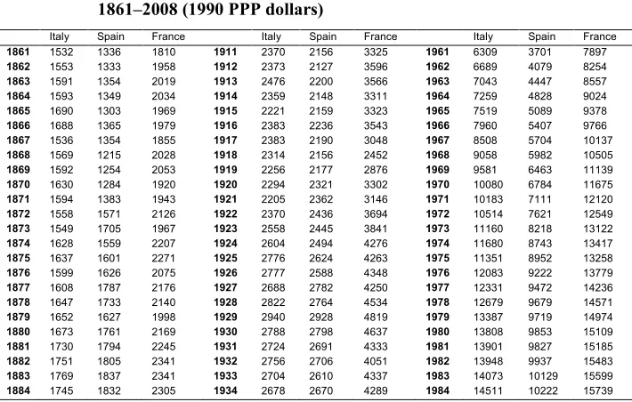
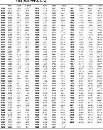
The series of GDP per capita at constant prices – expressed in 1990 international purchasing power parity (PPP) dollars – of Italy, Spain, and France are displayed in Figure 1.14 The series are expressed in natural logarithms in the upper part and in
inter-country ratios in the lower part. To visually highlight the long-run trends in the series, the years around the wars (1914–1919 and 1936–1946), characterized by very high short-run variance, are not shown. These years are, however, considered in the following analyses.
Figure 1: Per capita GDP in France, Italy, and Spain, 1861‒2008
Sources: Table A-1.
Natural logs 7 7,5 8 8,5 9 9,5 10 10,5 18 61 18 66 18 71 18 76 18 81 18 86 18 91 18 96 19 01 19 06 19 11 19 16 19 21 19 26 19 31 19 36 19 41 19 46 19 51 19 56 19 61 19 66 19 71 19 76 19 81 19 86 19 91 19 96 20 01 20 06 Years 1990 K -S d ol lar s France Italy Spain
Ratios (from original values)
40 50 60 70 80 90 100 110 120
The history of the ‘race’ in GDP between Italy and Spain can be summarized as follows. Italy began at a higher level, but lost some ground in the first decade after unification, and then from the end of the 19th century until the Spanish Civil War it had
a slight edge, although experiencing ups and downs. For fifteen years (1946–1961) after the Second World War the Italian advantage over Spain increased dramatically, but from the early 1960s Spain and Italy began to converge. Further insight comes from a comparison with France, as shown in the bottom part of Figure 1. Until the second half of the 20th century both Italy and Spain were declining, relative to France. Italy fell
behind until 1899, thereafter remaining more or less stable, whereas Spain continued to lose ground until 1960. However, in the second half of the 20th century the two
countries began steadily to converge, first Italy, then Spain. By the mid-1990s Italy had almost drawn equal with France, but from 2001 onwards it fell behind again, while conversely Spain continued to converge until 2008.15
To sum up, until the Second World War, Italy was confined to the status of the European periphery and was much closer to Spain than to France. In the second half of the 20th century its status became that of the European core; however, this status is now
in doubt (Felice and Vecchi 2015a). Spain began to converge towards the European core later, but its catching-up only came to a halt with the economic crisis.
It is interesting to compare GDP with life expectancy. The new series of this variable for Italy and Spain and that already available for France are shown in Figure 2 (the years around the wars, 1914–1919 and 1936−1946, are not shown). In contrast to GDP, at the beginning, i.e., through the first decades after Italy’s unification until the end of the 19th century, in life expectancy Italy’s advantage over Spain increased.
However, a second and maybe more important difference from the previous results is that Spain began to converge at the beginning of the 20th century and its life expectancy
caught up with Italy’s in the 1960s;16 i.e., much earlier than its convergence in GDP.
This result differs from what previous life expectancy data for Spain has suggested, that Spain began converging fifteen years earlier, around the second half of the 1880s, and stopped some years earlier, in the decade following the Second World War. This discrepancy is due to the fact that the official censuses, and even HMD data until 1930, under-reported infant mortality (for further details, see the online statistical appendix). Lastly, it should be noted that in the second half of the 1990s there was a new ‘reversal of fortunes’ in terms of life expectancy, with Italy once again taking the lead.
In broad terms, there are two important similarities between the patterns of GDP per capita and those of life expectancy: the initial advantage of Italy and the convergence of Spain over the long run. However, it is equally clear that the two indicators differ in at least two important respects. First, Spain began to converge sooner in life expectancy, and even overtook Italy as early as the 1960s when its convergence in per capita GDP had only just begun; second, Italy in turn again overtook Spain in life expectancy in the late 1990s, that is, at the same time as the Spanish convergence in per capita GDP accelerated remarkably.
Figure 2: Life expectancy in France, Italy, and Spain, 1861‒2008
When comparing Italy and Spain’s life expectancy with that of France, it emerges that around 1861 France had an even greater lead over Italy in life expectancy than it did in GDP. Italy, however, began to converge soon, starting in 1863, and had caught up with France by the mid-1950s, soon after convergence in GDP had begun and well before it was completed. This is similar to what we have seen for Spain in comparison with Italy. During the last decades, Italy continued to improve its position in life expectancy with respect to France, and had surpassed France by 1999. Conversely, Spain endured more ups and downs and began to steadily converge towards France later than Italy, in the last years of the 19th century, and reached the same level as France
roughly a decade after Italy did, in the middle of the 1960s. At the beginning of the 1970s, Spain also overtook France, and managed to maintain its lead throughout the 1980s. During the last two decades, Spain and France have ranked at practically the
same level, although Spain has been falling slightly behind − once again, in sharp
contrast with the GDP series. It may be worth adding that the convergence of Spain also took place in a wide range of other indicators of wellbeing, from height,17 to per capita
calories,18 to composite indicators such as the Human Development Index. With respect
to education, Spain has overtaken Italy in the last few years.19
From these comparisons, two regularities or common features emerge in the patterns of GDP and life expectancy. The first is the starting point. Differences in GDP mirror those in life expectancy at lower levels of socioeconomic development. At early stages a clear lead in GDP results in a clear lead in life expectancy, and vice versa. This finding is not new: in past historical periods when material conditions were dire and significant breakthroughs in medicine and social conditions had not yet taken place, there was a strong correlation between life expectancy and income in poor countries (e.g., Fogel 2004).20 The second regularity concerns the trend: in both Italy and Spain,
convergence in life expectancy begins earlier than in GDP. Life expectancy converges when the leading country (France in the case of Italy, and Italy in the case of Spain) is in the upward curve of its industrial transformation (which in its early stages may well have negative consequences for life expectancy). At the same time, the follower benefits from declining mortality due to breakthroughs in medicine and social conditions, but has not yet embarked on industrial transformation. This finding is in line
17 For Italy, see A’Hearn, Peracchi, and Vecchi (2009: 12−13); for Spain, see María-Dolores and Martínez-Carrión (2011: 35) and Martínez-Martínez-Carrión and Puche-Gil (2011: 444 and 447).
18 For Italy, see Sorrentino and Vecchi (2011: 12); for Spain, see Cussó Segura (2005). 19 For Italy, see Felice and Vasta (2015); for Spain, see Prados de la Escosura (2010b).
with literature showing that − in modern times − it is possible to reach high levels of
life expectancy even at relatively low levels of GDP (Caldwell 1986; Riley 2005).21
Of course, life expectancy is a highly synthetic indicator, whose evolution can be better understood by looking at its specific components. A primary issue is sex difference, where the three countries show remarkable similarities. They all record higher longevity for women, and with a similar advantage over men, growing from about one year at the beginning of the period to around six years at the end (HMD 2011a, 2011b, 2011c; Cabré, Domingo, and Menacho 2002; Blanes Llorens 2007). By contrast, age differences in mortality confirm the major backwardness of Italy and above all of Spain with respect to France, especially concerning mortality between the first and the third years of life (Ramiro Fariñas and Sanz Gimeno 2000a). As is well known, until the 20th century much of the increase in life expectancy at birth nearly
everywhere was a consequence of falling infant and child mortality rates. In absolute terms, this is true also for Italy and Spain. In addition, there are some broad features common to all continental Europe, despite the differences in level. Around the 1870s childhood mortality began to decline. In the interwar years, thanks to public health measures and the construction of urban infrastructure, the ratio of urban/rural mortality also started to fall. Then, after the Second World War, the spread of modern medicine and the advent of antibiotics further contributed to this process (e.g., Cutler, Deaton, and Lleras-Muney 2006; Livi-Bacci 2012).22 However, in terms of convergence, Spain,
and to a lesser degree Italy, began to catch up later. In terms of infant mortality, Spain started to converge only after 1960 (Nicolau 1989: 57 and 70–72). In Italy, convergence in infant mortality had begun in the second half of the 19th century and accelerated in
the second half of the 20th century (Felice 2007: 115). These different paces seem to be
at least partly related to the relative economic backwardness of the two countries. In Spain, for instance, the agrarian regions were, in demographic terms, more important than in Italy.23 Apart from lower average incomes, agrarian regions endured lower
hygienic and nutritional standards than the industrial areas, with consequences for
21 Not only for the reasons sketched above, but also thanks to other advances in social conditions such as improvements in literacy and education, especially among women (Riley 2001: 200−219). Literacy and education are omitted variables in our study, worthy of more investigation in the future (as far as we can tell at the present stage, their inclusion will further corroborate our findings).
22 For a recent and highly detailed analysis of these dynamics for the Spanish case, see Pérez Moreda, Reher, and Sanz Gimeno (2015: 79–248).
mortality levels.24 A similar case can be made for the convergence of Southern Italy,
whose mortality trends, when compared to the Centre-North of the peninsula (Felice and Vasta 2015), display features similar to those of Spain.
But the timing of the decline in infant mortality is also linked to a broader issue, a crucial one in the theoretical literature on the relation between life expectancy and GDP: the first demographic transition. France was the first country to undergo a demographic transition. There, the demographic transition began in the 19th century and
was completed in the first half of the 20th. In Italy, it lasted approximately from 1876 to
1965, as it did in other European countries such as Germany (Chesnay 1986: 294 and 301; Livi-Bacci 2012: 118). Conversely, in Spain the demographic transition was completed only during the 1980s (Carreras and Tafunell 2004: 38). A slower demographic transition means higher fertility rates and thus higher infant mortality. It may also have an impact on the relationship between life expectancy and GDP, as argued by the unified growth literature.
3. Trends in GDP and life expectancy
Thus far, we have considered GDP and life expectancy separately. However, in order to properly relate GDP and life expectancy, some transformations of the original values are required.
Life expectancy is a bounded variable: It has asymptotic limits that result from biological features (which may only be modified, and probably only to a certain extent, much more slowly than the time frame considered here). As a consequence, when its original values are employed, as life expectancy increases identical absolute changes result in lower increases. Specifically, when its starting level is lower, life expectancy mainly rises because of reductions in infant mortality; when its level is higher, it mainly falls among the elderly, but this has a minor impact on its rate of change. In short, the use of the original values implicitly assigns a higher weight to mortality reductions early in life (Deaton 2006); that is to say, it gives “more weight to saving the life of the younger over older people” (Prados de la Escosura 2014, p. 4). A solution was proposed by Kakwani (1993) and was adopted by Prados de la Escosura (2014), among others, via an achievement function that ensures that – so to speak – returns to increases in life expectancy do not decrease at higher levels. Accordingly, we compute Kakwani-transformed life expectancy (LEk) following the formula:
𝐿𝐸𝑘 =[𝑙𝑜𝑔(𝑀−𝑀0)−𝑙𝑜𝑔(𝑀−𝑥)]
𝑙𝑜𝑔(𝑀−𝑀0) (1)
where M is a maximum goalpost (83.2), M0 is a minimum goalpost (20), x is the value
of life expectancy, and log stands for the natural logarithm.25
By contrast, the GDP is an explosive rather than a bounded variable (at least in the period considered here). Thus, for time series analyses it is usually convenient to adopt a log transformation on its original values (Sen and Anand 2000), as we did in Figure 1.26 In the economic literature a common justification for this practice is that in the case
of GDP, as opposed to life expectancy, returns to well-being, or to the quality of life, are most likely to decline as the variable grows (Palazzi and Lauri 1998; Casadio Tarabusi, and Palazzi 2004; and, for the case of Italy, Sylos Labini 2014).
Figure 3 compares income and life expectancy for Italy, Spain, and France, making use of a natural log transformation for income and of a Kakwani transformation for life expectancy. Transformed GDP grew more than transformed life expectancy over the 1861‒2008 period, even though our transformation increases the growth rate of life expectancy and decreases that of GDP. However, life expectancy accelerated its growth in the last decades, when, conversely, GDP began slowing down. Unlike the previous result, this would not have emerged had we kept the original figures for income and life expectancy.
Beside these two common broad trends, there are significant cyclical differences between the three countries, which appear to be somehow related to their different levels of socioeconomic development. In Italy, GDP grew more than life expectancy from the end of the 19th century until the 1970s; later on, it was life expectancy (or,
better, achievements in longevity) that grew faster. For France we observe the same relationship, but significantly reinforced. In Spain, which was more backward, GDP grew more than life expectancy from the second half of the 19th century until the Civil
War. Then, in the first two decades of Franco’s regime, life expectancy grew at a faster rate than income. From the 1960s, GDP again grew faster than life expectancy, and this has only begun to change in the last few decades.
25 For the Kakwani transformation, we thus use the same thresholds as in Prados de la Escosura (2014, 2013), which are in turn obtained from the United Nations Development Programme (UNDP) (2010). In the UNDP reports from 1995 to 2009 the maximum and minimum values for life expectancy at birth were respectively established at 85 and 25 years. In the UNDP (2011) the maximum has been updated to 83.4 years (the new highest observed value). We tested the use of 85 years as a maximum and, as expected, results do not change significantly (they are available from the authors upon request).
Figure 3: Income and life expectancy in Italy, Spain, and France, 1861‒2008 Italy 7,0 7,5 8,0 8,5 9,0 9,5 10,0 10,5 18
61 1866 1871 1876 1881 1886 1891 9618 1901 1906 1911 1916 1921 1926 1931 1936 1941 1946 1951 1956 1961 1966 7119 1976 1981 1986 1991 1996 2001 2006
Years GD P 3,00 3,25 3,50 3,75 4,00 4,25 4,50 4,75 Lif e e xpe cta ncy GDP Life expectancy Spain 7,0 7,5 8,0 8,5 9,0 9,5 10,0 10,5 186 1 186 6 187 1 187 6 188 1 188 6 189 1 189 6 190 1 190 6 191 1 191 6 192 1 192 6 193 1 193 6 194 1 194 6 195 1 195 6 196 1 196 6 197 1 197 6 198 1 198 6 199 1 199 6 200 1 200 6 Years GD P 3,00 3,25 3,50 3,75 4,00 4,25 4,50 4,75 Lif e e xpe cta ncy GDP Life expectancy France 7,0 7,5 8,0 8,5 9,0 9,5 10,0 10,5 18
61 1866 1871 1876 1881 1886 1891 9618 1901 1906 1911 1916 1921 1926 1931 1936 1941 1946 1951 1956 1961 1966 7119 1976 1981 1986 1991 1996 2001 2006
4. Time series analysis
4.1 Granger causality
In order to formally analyse the correlation between life expectancy and GDP, it is first necessary to investigate their order of integration. As shown in Table A-5 in the online statistical appendix, augmented Dickey-Fuller tests show that it is necessary to produce first-differences of all series in order to make them stationary, i.e., all series exhibit a unit root. As a consequence, descriptive statistics of the simple correlation between GDP and life expectancy (as shown in the correlograms in Figure 4)27 necessarily
highlight a strong comovement of the series, with marked cross-correlation in all countries even extending over a 20-year interval.
However, such correlation does not imply that the series are indeed related, since integration of the first order implies that all series grow in time, possibly within an overall process of socioeconomic development. By contrast, consideration of the first differences of the series produces much less obvious results (as shown in Figure 4c). Thus, in the rest of the analysis, both series will always be considered in their first differences (denoted by ∆).
In order to investigate the relation between GDP and life expectancy we make recourse to the concept of Granger-causality, well known to economists. As shown below, Granger causality tests allow us to check for systematic short-run correlations between life expectancy and GDP. However, it should preliminarily be noted that the two series may well exhibit longer-term relations, for instance, via health investments made much earlier in life. A time-series analysis can hardly capture this effect: To this end a cross-sectional analysis based on a larger sample of countries (even though necessarily with less measurement accuracy than is possible here) would probably be more informative. Thus, our approach should be regarded as complementary to the more diffused approaches reviewed in Section 1, rather than as an alternative.
27 Given two series xi and yi, with i = 1, 2, … N-1, the cross-correlation r at delay d is defined as:
) ( ) ( )] ( ) [( 2 2 1 1 y y x x y y x x d i i d i i r N i − − ∑ − × − − × − = − =
Figure 4: Cross-correlations of GDP and life expectancy
Figure 4a) – GDP and modified LE
Figure 4b) – GDP and ln (LE)
Figure 4c) – GDP and modified LE: first differences
Intuitively, a variable x is said to Granger-cause another variable, y, if x systematically anticipates y in time. That is to say, x is considered to be the cause of y if the values of y can be better predicted by using past values of x (and possibly y too) than by using past values of y alone.28 It is customary to test for the presence of Granger
causality by regressing y on lagged values of y and x (Stock and Watson 2007). Wald statistics are then obtained, under the hypothesis that all coefficients on the lags of variable x are jointly zero in the equation for variable y.
However, since we are interested in both directions of causality, we run a vector regression (VR), allowing for up to four time lags (denoted here by j) for both variables. As already mentioned, we consider both LE and GDP (denoted by Y) in first differences, in order to investigate stationary series:
�∆𝐿𝐸∆𝑌𝑡=𝛼+∑ 𝛽4𝑗 𝑗∙ ∆𝐿𝐸𝑡−𝑗+∑ 𝛾4𝑗 𝑗∙ ∆𝑌𝑡−𝑗+𝜀𝑡
𝑡=𝛿+∑ 𝜗4𝑗 𝑗∙ ∆𝐿𝐸𝑡−𝑗+∑ 𝜑4𝑗 𝑗∙ ∆𝑌𝑡−𝑗+𝑢𝑡 (2) where the use of vector regression allows for the possible correlation between εt and ut. We separately test the two null hypotheses that all the coefficients that express the impact of one variable on the other (the four γjs and the four φjs) are not significantly different from zero, i.e., there is no Granger causality. The alternative hypothesis is that at least one coefficient is statistically different from zero (thus Granger causality cannot be excluded at the conventional thresholds of confidence). Accordingly, the test statistics is a Wald χ2 with 4 degrees of freedom. Results are shown in the two left-hand
columns of Table 1.
Overall, Granger causality tests of the relation between GDP growth and life expectancy are inconclusive. In most cases it emerges that no series has a statistically significant impact on the other at any time lag (up to four). The exceptions are Italy when using the natural logarithm of life expectancy rather than our modified index (this is done as a robustness check: see above, Section 3), and Spain, in the direction from GDP to life expectancy.
Table 1: Tests for Granger causality
VAR estimation Acemoglu-Johnson
Wald χ2(4) p-value IV coeff. Std. Err.
Italy GDP Granger-causes Modified LE 2.4412 0.655 0.032 0.034
Modified LE Granger-causes GDP 14.45 0.006 0.571 0.267
Spain GDP Granger-causes Modified LE 11.89 0.018 0.045 0.026
Modified LE Granger-causes GDP 2.0774 0.722 0.013 0.331
France GDP Granger-causes Modified LE 4.2224 0.377 0.047 0.036
Modified LE Granger-causes GDP 5.6425 0.227 -0.084 0.304
Note: bold values denote statistically significant coefficients, i.e., Granger causality cannot be refuted. For the second-step regressions in Acemoglu-Johnson estimates, see Table A-6 in the online statistical appendix.
Traditionally, economists think that such mixed results may arise due to possible endogeneity of the independent variables. Even though there is hardly reason to believe that GDP changes may be a consequence of LE developments – which they nonetheless anticipate in time – or vice versa, this has been claimed (e.g., Acemoglu and Johnson 2007). They thus propose coping with this possible endogeneity using an instrumental variables approach (IV), adopting as instruments the second differences of LE and GDP, the third differences, and so on (respectively denoted by ∆2 and ∆3, etc.).
Thus, as a robustness check we run such models, but due to computational and data limitations we limit the analysis to causality with one time lag, as shown below (variables with a hat denote predicted values):
�∆𝐿𝐸𝑡=𝜇+∑ 𝛽𝑗4 𝑗∙ ∆𝐿𝐸𝑡−𝑗+𝜁 ∙ ∆𝑌�𝑡−1+𝜀𝑡
∆𝑌𝑡=𝜂+𝜆 ∙ ∆𝐿𝐸�𝑡−1+∑ 𝜑4𝑗 𝑗∙ ∆𝑌𝑡−𝑗+𝑢𝑡 (3)
Thus the first stage regressions are:
⎩ ⎪ ⎨ ⎪
⎧∆𝐿𝐸𝑡−1=𝑎+� 𝜓𝑗∙ ∆𝑌𝑡−𝑗
4
𝑗
+𝑏 ∙ ∆2𝐿𝐸
𝑡−1+𝑐 ∙ ∆3𝐿𝐸𝑡−1+𝑑 ∙ ∆4𝐿𝐸𝑡−1+𝑒 ∙ ∆5𝐿𝐸𝑡−1+𝜀𝑡
∆𝑌𝑡−1=𝑓+� 𝜏𝑗∙ ∆𝐿𝐸𝑡−𝑗
4
𝑗
+𝑔 ∙ ∆2𝑌𝑡−1+ℎ ∙ ∆3𝑌𝑡−1+𝑘 ∙ ∆4𝑌𝑡−1+𝑙 ∙ ∆5𝑌𝑡−1+𝑢𝑡
(4)
case (full results are reported in Table A-6 in the online statistical annex). Indeed, the IV procedure returns similar results to the VR estimation in terms of the statistical significance of the coefficients of interest (i.e., we cannot reject Granger causality only of LE on GDP for Italy, and of GDP on LE for Spain). Thus, in both models (VR and IV estimations) the lack of consistent results prevents us from identifying a stable and consistent causality relation between life expectancy and GDP, which is problematic from the point of view of the unified growth theory.
One possible explanation for this lack of consistency is that the relation between the two variables is non-monotonic but rather changes over time. In order to investigate this possibility, we investigate the series for possible structural breaks, i.e., points beyond which it may be said that a series exhibits a significantly different pattern (e.g., a different long-run trend) and which therefore define periods that – at least for some empirical applications – should be considered separately.
4.2 Structural breaks and sub-period Granger causality
In order to detect whether there are any breaks in the series, in this section we adopt an ex-post periodization. We use the well-known test developed by Bai and Perron (1998, 2003). As shown in Table A-7 in the online statistical appendix, frequently, though not consistently, the identification of several breaks fits the data better in terms of the sum of squared residuals. In the extreme, treating each year as unique would produce the best historical explanation. However, reasons of parsimony in choosing the explicative model induce us to weigh the information that additional variables provide against the complexity that they introduce into our model.
To this end, a common approach is to select the number of breaks that maximizes the Bayesian Information Criterion (BIC). Excluding the cases of four or more breaks, for all series the local maximum of the BIC corresponds to zero structural breaks. This does not imply that the series necessarily exhibit no structural breaks, but rather that, taken in isolation, the information that can be obtained from considering these breaks would not compensate for the complexity that they introduce into the model. However, since the aim of this section is to prudentially investigate whether structural breaks may induce the mixed results concerning Granger causality that we discussed above, for all series we consider at least one break.29 This can therefore be considered as a robustness
check of the previous analysis.
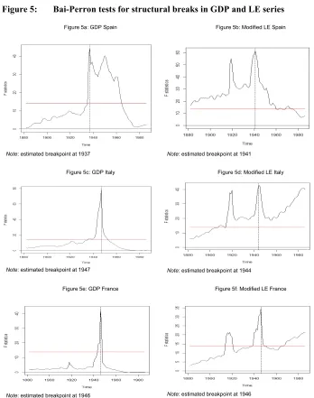
As shown in Figure 5, according to the Bai-Perron tests the breaks that best describe the series (peak values of the F statistics) are: 1946 for both modified LE and GDP in France, respectively 1944 and 1947 for Italy, and respectively 1941 and 1937 for Spain. As shown in Table A-8 in the online statistical appendix, further tests for exogenous breaks, following Prados de la Escosura (2003), confirm the same breaks for the three countries.
Thus, we identify structural breaks in both life expectancy and GDP roughly corresponding to the Second World War for Italy and France and to the Civil War for Spain. For Italy, as is well known, the end of the Second World War marked the beginning of a period of unprecedented growth – the “economic miracle” − which
brought the country back “from the periphery to the centre” (Zamagni 1993) as the sixth world economic power, and which saw remarkable improvements in social indicators and well-being (Felice and Vecchi 2015b). The misalignment of breaks in the Spanish series may arise from the peculiarity of the country’s socioeconomic development, and may be interpreted as a manifestation of its underdevelopment in the early and mid-20th
century, until well into the 1960s.30
here we are interested in prudentially investigating – as a robustness check of the previous analysis – whether such acceleration(s), beyond a certain threshold, should be regarded as defining two periods that should be kept separate in empirical applications, and specifically whether they could induce us to falsely reject causality between LE and GDP.
Figure 5: Bai-Perron tests for structural breaks in GDP and LE series
Figure 5a: GDP Spain
Note: estimated breakpoint at 1937
Figure 5b: Modified LE Spain
Note: estimated breakpoint at 1941
Figure 5c: GDP Italy
Note: estimated breakpoint at 1947
Figure 5d: Modified LE Italy
Note: estimated breakpoint at 1944
Figure 5e: GDP France
Note: estimated breakpoint at 1946
Figure 5f: Modified LE France
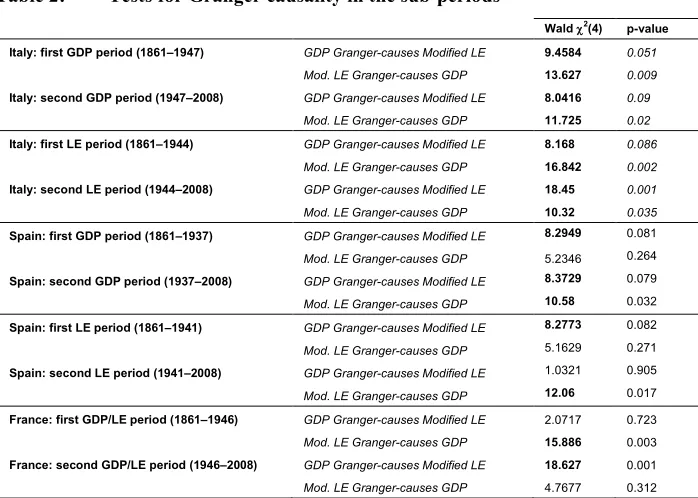
Repeating the tests of Granger causality for the sub-periods identified by these breaks, as shown in Table 2, helps us clarifying a number of crucial issues. In the first period, which can be identified with economic backwardness, economic growth consistently Granger-causes improvements in life expectancy in Spain and Italy, but not in France, the country with the highest levels of GDP and LE and the lowest LE growth. The reverse, i.e., that improvements in life expectancy Granger-cause GDP growth, seems to be true in Italy and in France for this period, but not in Spain, i.e., in the country with the lowest level of GDP and LE. In the second period, i.e., after the Second World War for Italy and France and after the Civil War for Spain, the bidirectional Granger-causality is confirmed for Italy and partially for Spain (although for Spain such a result crucially depends on the specific periodization used – i.e., if the 1941 break is included or not in this second period – and therefore the result cannot be considered as very robust). By contrast, for France we observe an inversion of statistical significance, with GDP growth now predicting LE improvements, while improvements in LE no longer predict GDP growth.
Table 2: Tests for Granger causality in the sub-periods
Wald χ2(4) p-value
Italy: first GDP period (1861‒1947) GDP Granger-causes Modified LE 9.4584 0.051
Mod. LE Granger-causes GDP 13.627 0.009
Italy: second GDP period (1947‒2008) GDP Granger-causes Modified LE 8.0416 0.09
Mod. LE Granger-causes GDP 11.725 0.02
Italy: first LE period (1861‒1944) GDP Granger-causes Modified LE 8.168 0.086
Mod. LE Granger-causes GDP 16.842 0.002
Italy: second LE period (1944‒2008) GDP Granger-causes Modified LE 18.45 0.001
Mod. LE Granger-causes GDP 10.32 0.035
Spain: first GDP period (1861‒1937) GDP Granger-causes Modified LE 8.2949 0.081
Mod. LE Granger-causes GDP 5.2346 0.264
Spain: second GDP period (1937‒2008) GDP Granger-causes Modified LE 8.3729 0.079
Mod. LE Granger-causes GDP 10.58 0.032
Spain: first LE period (1861‒1941) GDP Granger-causes Modified LE 8.2773 0.082
Mod. LE Granger-causes GDP 5.1629 0.271
Spain: second LE period (1941‒2008) GDP Granger-causes Modified LE 1.0321 0.905
Mod. LE Granger-causes GDP 12.06 0.017
France: first GDP/LE period (1861‒1946) GDP Granger-causes Modified LE 2.0717 0.723
Mod. LE Granger-causes GDP 15.886 0.003
France: second GDP/LE period (1946‒2008) GDP Granger-causes Modified LE 18.627 0.001
Mod. LE Granger-causes GDP 4.7677 0.312
We may sum up the results as follows. Improvements in life expectancy seem to predict GDP growth, but with two exceptions: Spain in the first period, i.e., the country with lower levels of GDP and life expectancy and a delayed demographic transition; and France in the second period, i.e., the country with higher GDP and life expectancy (and slower growth). Economic growth consistently Granger-causes improvements in modified life expectancy, with one important exception: France in the first period, i.e., the country with the earliest demographic transition, where improvements in life expectancy appear to be slower and independent of economic growth.
By combining these results with the analysis in the previous Section (see Figure 3), some important points arise regarding the correlation between GDP and life expectancy. One issue is the causality going from life expectancy to income, concerning which we can detect three phases. In the first, there does not seem to be a significant contribution of life expectancy to income: The initial rise in income is independent of improvements in life expectancy. In the second phase, improvements in life expectancy do seem to lead to further advances in GDP. The movements in these first two phases are compatible with the unified growth theory, which stresses a positive impact of improvements in life expectancy upon economic growth only after the onset of the demographic transition (Galor and Weil 2000; Cervellati and Sunde 2011). In a third phase, when a negative link (or at least a non-positive one) from life expectancy to GDP seems to emerge: Very high life expectancy may result in a disproportionately old population, which may hamper economic growth. Such an outcome, in line with what has been found for other countries such as the United States (Eggleston and Fuchs 2012), was not predicted by the unified growth theory.
Concerning the impact of income on life expectancy, it is commonly held that at the early stages GDP significantly impacts upon life expectancy. By analysing the historical data for 16 Western countries in benchmark years from 1870 to 2000, Livi-Bacci (2012, p. 125) has simplified the rationale as follows: “more food, better clothing, better houses, and more medical care have a notable effect on those who are malnourished, badly clothed, poorly housed, and forced to trust fate in case of sickness”. Regarding later phases, it has been argued that when a rise in per capita GDP benefits an already prosperous population the effects on life expectancy are minimal, and may even be negative if GDP growth comes at the detriment of environmental conditions.31 Once a Kakwani transformation is employed in order to properly account
for achievements in longevity − that is, once we eliminate the bias in favour of infant
mortality and treat more fairly the improvements in longevity of the elderly
population – only the first of these assumptions is supported by our findings, and even with the important exception of France (possibly because it already enjoyed a relatively high life expectancy which tended to grow less, as a consequence of an early demographic transition). A positive impact of GDP on life expectancy is also found for the following period, when GDP significantly increased.
On the whole, these results show that the heterogeneity in the relation between life expectancy and GDP growth that was found for the entire series may indeed depend on the existence of structural breaks. However, the specific historical experience of each country is important too: Within a general framework, country-specific historical idiosyncrasies should not be overlooked.
5. Conclusions
After reviewing and updating the available estimates, we presented and discussed long-run (1861–2008) series of per capita GDP and life expectancy for Italy and Spain and compared them with those available for France, their common and most important neighbouring country. Our goal was not only to briefly reconsider the economic history of the two countries in the light of the new time series evidence, but also to investigate the long-run evolution of per capita GDP and life expectancy and their mutual relationship, by way of country case studies and a time-series approach.
We find evidence, or confirmation, of three common features in the patterns of per capita GDP and life expectancy. First, at early stages of socioeconomic development, when both GDP and life expectancy are low, the differences in GDP mirror those in life expectancy: A clear lead in GDP results in a clear lead in life expectancy. Second, in the long run, convergence is confirmed for both indicators (significant cyclical differences notwithstanding): At the beginning of the period, Spain is the most backward country in both life expectancy and GDP, but over the entire period it is also the country converging at the highest average rate, while Italy ranks in the middle between Spain and France. Third, convergence in life expectancy tends to begin earlier than convergence in GDP: Spain caught up with Italy earlier in life expectancy than in GDP, and both countries caught up with France earlier in life expectancy than in GDP.
Concerning the causal link from life expectancy to income, our findings may be explained by the existence of a non-monotonic relationship between the two variables. In line with recent results from unified growth theory, before the onset of the demographic transition it seems that there is no significant impact of life expectancy on income, whereas after the demographic transition improvements in life expectancy lead to further advances in GDP. More recently, however, a third phase appears to emerge, characterized by a negative link from (very high) life expectancy to GDP. Such a finding cannot be explained in terms of the unified growth theory and deserves further study.
Finally, concerning the link from income to life expectancy, once the latter is transformed in order to properly account for achievements in longevity, we find evidence of a positive and consistent impact of GDP on life expectancy. However, an exception must be made for France, which experienced an early demographic transition.
In conclusion, our findings confirm the importance of a general theoretical framework in order to address the correlation between life expectancy and GDP, such as that proposed by the unified growth theory. However, they also suggest that the peculiarity of each historical case should not be ignored.
6. Acknowledgments
References
A’Hearn, B., Peracchi, F., and Vecchi, G. (2009). Height and the normal distribution: Evidence from Italian military data. Demography 46(1): 1‒25. doi:10.1353/ dem.0.0049.
Acemoglu, D. and Johnson, S. (2007). Disease and development: The effect of life expectancy on economic growth. Journal of Political Economy 115(6): 925‒985. doi:10.1086/529000.
Alessandrini, P. and Fratianni, M. (2015). In the absence of fiscal union, the Eurozone needs a more flexible monetary policy. PSL Quarterly Review 68(275): 279‒
296.
Altug, S., Filiztekin, A., and Pamuk, S. (2008). Sources of long-term economic growth for Turkey, 1880–2005. European Review of Economic History 12(3): 393‒430. doi:10.1017/S1361491608002293.
Andrews, D.W.K. (1993). Tests of parameter instability and structural change with unknown change point. Econometrica59(3): 821‒856.doi:10.2307/2951764. Arbelo Curbelo, A. (1951). Necesidad demográfico-sanitaria de rectificar el concepto
legal de nacido vivo. Revista Internacional de Sociología 9(36): 393‒405. Baffigi, A. (2011). Italian national accounts, 1861‒2011. Rome: Banca d’Italia
(Quaderni di Storia Economica; no. 18).
Bai, J., and Perron, P. (1998). Estimating and testing linear models with multiple structural changes. Econometrica 66(1): 47‒78. doi:10.2307/2998540.
Bai, J., and Perron, P. (2003). Computation and analysis of multiple structural change model. Journal of Applied Econometrics 18(1): 1‒22. doi:10.1002/jae.659. Battilani, P., Felice, E., and Zamagni, V. (2014). Il valore aggiunto dei servizi a prezzi
correnti (1861‒1951). Rome: Banca d’Italia (Quaderni di Storia Economica, no. 33).
Ben-David, D. and Papell, D.H. (2000). Some evidence on the continuity of the growth process among the G7 countries. Economic Inquiry 38(2): 320‒330. doi:10.11 11/j.1465-7295.2000.tb00020.x.
Blanes Llorens, A. (2007). La mortalidad en la España del siglo XX. Análisis demográfico y territorial [Ph.D. thesis]. Barcelona: Universitat Autònoma de Barcelona, Department de Geografia, Facultat de Filosofia i Lletres.
Botti, F., Corsi, M., and D’Ippoliti, C. (2016). The gendered nature of poverty in the EU: Individualized versus collective poverty measures. Feminist Economics
22(4): 82‒110. doi:10.1080/13545701.2016.1146408.
Brandolini, A. and Vecchi, G. (2011). The well-being of Italians: A comparative historical approach. Rome: Banca d’Italia (Quaderni di Storia Economica; no. 19).
Brunello, G. and Labartino, G. (2014). Regional differences in overweight rates: The case of Italian regions. Economics and Human Biology 12(1): 20‒29. doi:10.10 16/j.ehb.2012.10.001.
Brunetti, A., Felice, E., and Vecchi, G. (2011). Reddito. In: Vecchi, G. (ed.). In ricchezza e in povertà: Il benessere degli italiani dall’Unità a oggi. Bologna: Il
Mulino: 209‒234 and 427‒429.
Cabré, A. (1999). El sistema català de reproducció. Barcelona: Proa, Institut Català de la Mediterrània d’Estudis i Cooperació.
Cabré, A., Domingo, A., and Menacho, T. (2002). Demografía y crecimiento de la población española durante el siglo XX. In: Pimentel Siles, M. (ed.). Mediterráneo económico, 1. monogràfic: Procesos migratorios, economía y personas. Almeria: Caja Rural Intermediterránea Cajamar: 121‒138.
Cahill, M.B. (2002). Diminishing returns to GDP and the Human Development Index. Applied Economic Letters 9(13): 885‒897. doi:10.1080/13504850210158999. Caldwell, J.C. (1986). Routes to low mortality in poor countries. Population and
Development Review 12(2): 171‒220. doi:10.2307/1973108.
Carreras, A. (1989). La industrialización española en el marco de la historia económica europea: Ritmos y caracteres comparados. In: García Delgado, J.L. (ed.). España, economía. Madrid: Espasa Calpe: 79‒115.
Carreras, A. (1990). Industrialización española: Estudios de historia cuantitativa. Madrid: Espasa Calpe.
Carreras, A. (1997). La industrialización: Una perspectiva de largo plazo. Papeles de Economía Española 73: 35‒60.
Carreras, A. and Felice, E. (2010). L’industria italiana dal 1911 al 1938: Ricostruzione della serie del valore aggiunto e interpretazioni. Rivista di Storia Economica
26(3): 285‒333.
Carreras, A. and Tafunell, X. (2004). Historia económica de la España contemporánea. Barcelona: Crítica.
Cervellati, M. and Sunde, U. (2011). Life expectancy and economic growth: The role of the demographic transition. Journal of Economic Growth 16(2): 99‒133. doi:10.1007/s10887-011-9065-2.
Chatfield, C. (1980). Theanalysis of time series: An introduction. 2nd edition. London:
Chapman and Hall. doi:10.1007/978-1-4899-2923-5.
Chesnay, J.-C. (1986). La transition démographique: Étapes, formes, implications économiques: Etude de séries temporelles (1720‒1984) relatives à 67 pays. Paris: PUF.
Comín, F. (1995). La difícil convergencia de la economía española: Un problema histórico. Papeles de Economía Española 63: 78‒92.
Costa-Font, J., Hernández-Quevedo, C., and Jiménez-Rubio, D. (2014). Income inequalities in unhealthy life styles in England and Spain. Economics and Human Biology 13(2): 66‒75. doi:10.1016/j.ehb.2013.03.003.
Crafts, N.F.R. (1997). The human development index and changes in standards of living: Some historical comparisons. European Review of Economic History 1(3): 299‒322. doi:10.1017/S1361491697000142.
Crafts, N.F.R. (2002). The human development index, 1870‒1999: Some revised estimates. European Review of Economic History 6(3): 395‒405. doi:10.1017/ S1361491602000187.
Crafts, N.F.R., Leybourne, S.J., and Mills, T.C. (1990). Measurement of trend growth in European industrial output before 1914: Methodological issues and new estimates. Explorations in Economic History 27(4): 442‒467. doi:10.1016/0014-4983(90)90024-S.
Cussó Segura, X. (2005). El estado nutritivo de la población española 1900‒1970. Análisis de las necesidades y disponibilidades de nutrientes. Historia Agraria 36: 329‒358.
Cutler, D., Deaton, A., and Lleras-Muney, A. (2006). The determinants of mortality. Journal of Economic Perspectives 20(3): 97‒120. doi:10.3386/w11963.
De Corso, G. (2013). El crecimiento económico de Venezuela, desde la oligarquía conservadora hasta la revolución bolivariana: 1830‒2012. Una visión cuantitativa. Revista de Historia Económica / Journal of Iberian and Latin American Economic History 31(3): 321‒357.
Dopico, F. (1987). Regional mortality tables for Spain in the 1860. Historical Methods 20(4): 173‒179. doi:10.1080/01615440.1987.9955273.
Dopico, F. and Reher, D.-S. (1999). El declive de la mortalidad en España, 1860–1930. Zaragoza: Asociación de Demografía Histórica (Monografías ADEH 1).
Egger, G., Swinburn, B., and Islam, A.F.M. (2012). Economic growth and obesity: An interesting relationship with world-wide implications. Economics and Human Biology 10(2): 147‒153. doi:10.1016/j.ehb.2012.01.002.
Eggleston, K.N. and Fuchs, V.R. (2012). The new demographic transition: Most gains in life expectancy now realized late in life. Journal of Economic Perspectives
26(3): 137‒156.doi:10.1257/jep.26.3.137.
Escudero, A. and Simón, H. (2010). Nuevos datos sobre el bienestar en España (1850‒
1993). In: Chastagnaret, G., Daumas, J.C., Escudero, A., and Raveux, O. (eds.). Los niveles de vida en España y Francia (siglos XVIII–XX). San Vicente del Raspeig: Publicaciones de la Universidad de Alicante: 213–252.
Felice, E. (2007). Divari regionali e intervento pubblico: Per una rilettura dello sviluppo in Italia. Bologna: Il Mulino.
Felice, E. (2010). Regional development: Reviewing the Italian mosaic. Journal of Modern Italian Studies 15(1): 64‒80. doi:10.1080/13545710903465556.
Felice, E. (2011). Regional value added in Italy, 1891‒2001, and the foundation of a long-term picture. Economic History Review 64(3): 929‒950. doi:10.1111/j.146 8-0289.2010.00568.x.
Felice, E. (2016). GDP and convergence in modern times. In: Diebolt, C. and Haupert, M. (eds.). Handbook of Cliometrics. Berlin: Springer: 263‒293. doi:10.1007/97 8-3-642-40458-0_5-2.
Felice, E. and Carreras, A. (2012). When did modernization begin? Italy’s industrial growth reconsidered in light of new value-added series, 1911−1951.
Explorations in Economic History 49(4): 443‒460. doi:10.1016/j.eeh.2012.07. 004.
Felice, E. and Pujol Andreu, J. (2013). GDP and life expectancy in Italy and Spain over the long-run (1861–2008): Insights from a time-series approach. Barcelona: Universitat Autònoma de Barcelona (UHE Working Paper 2013_06). http://www.h-economica.uab.es/wps/2013_06.pdf.
Felice, E. and Vecchi, G. (2015a). Italy’s growth and decline, 1861‒2011. Journal of Interdisciplinary History 45(4): 507‒548. doi:10.1162/JINH_a_00757.
Felice, E. and Vecchi, G. (2015b). Italy’s modern economic growth, 1861‒2011. Enterprise and Society 16(2): 225‒248. doi:10.1017/eso.2014.23.
Fenoaltea, S. (1969). Public policy and Italian industrial development, 1861–1913. Journal of Economic History 29(1): 176–179. doi:10.1017/S0022050700097898. Fenoaltea, S. (2003). Notes on the rate of industrial growth in Italy, 1861–1913. Journal of Economic History 63(3):695‒735. doi:10.1017/S0022050703541961. Fenoaltea, S. (2005). The growth of the Italian economy, 1861‒1913: Preliminary
second-generation estimates. European Review of Economic History 9(3): 273‒
312. doi:10.1017/S136149160500153X.
Fenoaltea, S. (2010). The reconstruction of historical national accounts: The case of Italy. PSL Quarterly Review 63(252): 77‒96.
Fenoaltea, S. (2011). The reinterpretation of Italian economic history: From unification to the Great War. Cambridge: Cambridge University Press. doi:10.1017/CBO97 80511730351.
Fogel, R.W. (2004). The escape from hunger and premature death, 1700‒2100: Europe, America and the Third World. Cambridge: Cambridge University Press. doi:10.1017/CBO9780511817649.
Fraile, P. (1991). Industrialización y grupos de presión: La economía política de la protección en España. Madrid: Alianza.
Gallup, J.L., Sachs, J.D., and Mellinger, A.D. (1999). Geography and economic development. International Regional Science Review 22(2): 179‒232. doi:10.11 77/016001799761012334.
Galor, O. (2012). The demographic transition: Causes and consequences. Cliometrica 6(1): 1‒28. doi:10.1007/s11698-011-0062-7.
Galor, O. and Weil, D.N. (2000). Population, technology, and growth: From Malthusian stagnation to the demographic transition and beyond. American Economic Review 90(4): 806‒828. doi:10.1257/aer.90.4.806.
Gerschenkron, A. (1947). The Soviet indices of industrial production. Review of Economics and Statistics 29(4): 217–226. doi:10.2307/1927819.
Glei, D.A., Gómez Redondo, R., Argüeso, A., and Canudas-Romo, V. (2012). About mortality data for Spain. Human Mortality Database. Rostock: Max Planck Institute for Demographic Research, and Berkeley: University of California. http://www.mortality.org/.
Goldstein, J.R., Kreyenfeld, M., Jasilioniene, A., and Örsal, D.K. (2013). Fertility reactions to the ‘Great Recession’ in Europe: Recent evidence from order-specific data. Demographic Research 29(4): 85‒104. doi:10.4054/DemRes.2013. 29.4.
Gómez Redondo, R. (1992). La mortalidad infantil española en el siglo XX. Madrid: CIS-Siglo XXI.
Granger, C.W.J. (1969). Investigating causal relations by econometric models and cross-spectral methods. Econometrica 37(3): 424‒438. doi:10.2307/1912791. Hernández Adell, I., Muñoz Pradas, F., and Pujol Andreu, J. (2013). Difusión del
consumo de leche en España (1865‒1981). Barcelona: Universitat Autònoma de Barcelona, Departament d’Economia i d’Història Econòmica (UHE Working Paper; 2013_03).
HMD (Human Mortality Database) (2011a). France, Total Population, Life expectancy at birth (period, 1x1). Human Mortality Database. Rostock: Max Planck Institute for Demographic Research, and Berkeley: University of California. http://www.mortality.org/.
HMD (Human Mortality Database) (2011b). Italy, Life expectancy at birth (period, 1x1). Human Mortality Database. Rostock: Max Planck Institute for Demographic Research, and Berkeley: University of California. http://www.mortality.org/.
HMD (Human Mortality Database) (2011c). Spain, Life expectancy at birth (period, 1x1). Human Mortality Database. Rostock: Max Planck Institute for Demographic Research, and Berkeley: University of California. http://www.mortality.org/.
Ine (Institudo Nacional de Estadística) (2012). Estimaciones de Población Actual de España. Resultados Nacionales. Madrid.
Istat (Istituto Centrale di Statistica) (1957). Indagine statistica sullo sviluppo del reddito nazionale dell’Italia dal 1861 al 1956. Rome: Istat (Annali di Statistica 8[9]). Istat (Istituto Centrale di Statistica) (2012a). Ricostruzione della popolazione residente
e del bilancio demografico. Rome: Istat.
Kakwani, N. (1993). Performance in living standards: An international comparison. Journal of Development Economics 41(2): 307‒336. doi:10.1016/0304-3878(93) 90061-Q.
Livi-Bacci, M. (2012). A concise history of world population. 5th edition. Oxford:
Blackwell.
Lorentzen, P., McMillan, J., and Wacziarg, R. (2008). Death and development. Journal of Economic Growth 13(2): 81‒124. doi:10.1007/s10887-008-9029-3.
Maddison, A. (1991). A revised estimate of Italian economic growth, 1861‒1989. BNL Quarterly Review 177: 225‒241.
Maddison, A. (2006). The world economy: A millennial perspective. Paris: OECD. doi:10.1787/9789264022621-en.
Maddison, A. (2010). Historical statistics of the world economy: 1‒2008 AD. Paris: OECD. www.ggdc.net/maddison/content/shtml.
Maluquer de Motes, J. (2008). El crecimiento moderno de la población de España de 1850 a 2001: Una serie homogénea anual. Investigaciones de Historia Económica (4)10: 129‒162. doi:10.1016/S1698-6989(08)70139-5.
Maluquer de Motes, J. (2009a). Del caos al cosmos: Una nueva serie enlazada del producto interior bruto de España entre 1850 y 2000. Revista de Economía Aplicada 17(49): 5‒45.
Maluquer de Motes, J. (2009b). Viajar a través del cosmos: La medida de la creación de la riqueza y la serie histórica del producto interior bruto de España (1850–2008). Revista de Economía Aplicada 17(51): 25–54.
María-Dolores, R. and Martínez-Carrión, J.M. (2011). The relationship between height and economic development in Spain, 1850‒1958. Economics and Human Biology, 9(1): 30‒44. doi:10.1016/j.ehb.2010.07.001.
Martínez-Carrión, J.M. and Puche-Gil, J. (2011). La evolución de la estatura en Francia y en España, 1770‒2000: Balance historiográfico y nuevas evidencias. Dynamis 31(2): 429‒452.
Molinas, C. and Prados de la Escosura, L. (1989). Was Spain different? Spanish historical backwardness revisited. Explorations in Economic History 26(4): 385‒
402. doi:10.1016/0014-4983(89)90015-6.
Nadal, J. and Sudrià, C. (1993). La controversia en torno al atraso económico español en la segunda mitad del siglo XIX (1860‒1913). Revista de Historia Industrial 3: 199‒227.
Nicolau, R. (2005). Población, salud y actividad. In: Carreras, A. and Tafunell, X. (eds.). Estadísticas históricas de España: Siglos XIX‒XX. Madrid: Fundación BBVA: 77‒154.
OECD (Organisation for Economic Co-operation and Development) (2014). OECD.Stat. http://stats.oecd.org.
Palazzi, P. and Lauri, A. (1998). The Human Development Index: Suggested corrections. Banca Nazionale del Lavoro Quarterly Review 51(205): 193‒221. Pascua Martínes, M. (1934). Mortalidad específica en España: I. Cálculo de
poblaciones. II. Mortalidad por sexos, grupos de edad y causas en el período 1911–1930. Madrid: Publicaciones oficiales de la CPIS.
Pérez Moreda, V., Reher, D.S., and Sanz Gimeno, A. (2015). La conquista de la salud: Mortalidad y modernización en la España contemporánea. Madrid: Marcial Pons Historia.
Pons, J. and Tirado, D. (2006). Discontinuidades en el crecimiento económico en el período 1870‒1994: España en perspectiva comparada. Revista de Economía Aplicada 40: 137‒156.
Prados de la Escosura, L. (1997). Política económica liberal y crecimiento en la España contemporánea: Un argumento contrafactual. Papeles de Economía Española 73: 83‒98.
Prados de la Escosura, L. (2000). International comparisons of real product,
1820−1990: An alternative data set. Explorations in Economic History 37(1): 1–
41. doi:10.1006/exeh.1999.0731.
Prados de la Escosura, L. (2003). El progreso económico de España (1850‒2000). Bilbao: Fundación BBVA.
Prados de la Escosura, L. (2007). European patterns of development in historical perspective. Scandinavian Economic History Review 55(3): 187‒221. doi:10.108 0/03585520701751640.
Prados de la Escosura, L. (2009). Del cosmos al caos: La serie del PIB de Maluquer de Motes. Revista de Economía Aplicada 17(51): 5–23.
Prados de la Escosura, L. (2010a). Spain’s international position, 1850‒1913. Revista de Historia Económica / Journal of Iberian and Latin American Economic History 28(1): 173‒215.