Unit 5
SIMULATION THEORY
Lesson 40
Learning objectives:
• To acquaint yourself with the practical applications of simulation methods.
Hello students,
Now when you are aware of the methods of simulation and techniques of random number generation I’ll take few examples of business / practical application of simulation. Simulation is widely used for the following
• Simulation of Inventory Problem
• Simulation of Queuing Problem
• Simulation of investment problem
• Simulation of Maintenance Problem
• Simulation of PERT Problem
Firstly, let us find out how simulation can be utilized for an inventory problem.
Simulation of Inventory Problem
followed by demand or supply. It is however possible to get the solution by using simulation techniques. The basic approach would be to determine the probability distribution of the input and output functions from the past data, and run the inventory system artificially by generating the future observations on the assumptions of the same distribution. Subsequently, the decision-making regarding the optimization problems would be made by the trial-and-error method.
Many companies are looking to reduce their inventory costs, however before risking adverse customer service they want to determine the consequences and test different alternatives. By building a model of the inventory system, we can test variations of the existing setup.
Example 1
Using the random number to simulate a sample, find the probability that a packet does not contain any defective product, when the production line produces 10% defective products. Compare your answer with the expected probability.
Solution
Given that 10 per cent of the total production is defective and 90 per cent is non-defective. If we have 100 random numbers (0 to 99), then 90 or 90 per cent of them represent non-defective products and remaining 10 (or 10 per cent) of them represent defective products. Thus, the random numbers 00 to 89 are assigned to variables representing non-defective products and 90 to 100 are assigned to variables representing defective products.
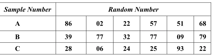
If we choose a set of 2-digit random numbers in the range 00 to 99 to represent a packet of 6 products as shown below, then we would expect that 90 per cent of the time they would fall in the range 00 to 89.
Table 1
Sample Number Random Number
A 86 02 22 57 51 68
B 39 77 32 77 09 79
D 97 66 63 99 61 80
E 69 30 16 09 05 53
F 33 63 99 19 87 26
G 87 14 77 43 96 43
H 99 53 93 61 28 52
I 93 86 52 77 65 15
J 18 46 23 34 25 85
Here it may be noted that out of ten simulated samples 6 contain one or more defectives and 4 contain no defectives. Thus, the expected percentage of non-defective products is 40 per cent. However theoretically the probability that a packet of 6 products containing no defective products is (0.9)6 = 0.53144 = 53.14%
Example 2
A bakery keeps stock of a popular brand of cake. Previous experience shows the demand pattern for the item with associated probabilities, as given below:
Daily demand (number): 0 10 20 30 40 50
Probability : 0.01 020 0.15 0.50 0.12 0.02
Use the following sequence of random numbers to simulate the demand for next 10 days.
Random numbers: 25, 39, 65, 76, 12, 05, 73, 89, 19, 49.
Solution
Using the daily demand distribution, we obtain a probability distribution as shown in the following table:
Table 2 Daily Demand Distribution
Daily Demand Probability Cumulative Random Number
Probability Interval
0 0.01 0.01 00
10 0.20 0.21 01-20
20 0.15 0.36 21-35
30 0.50 0.86 36-85
40 0.12 0.98 86-97
50 0.02 1.00 98-99
Conduct the simulation experiment for demand by taking a sample of 10 random numbers from a table of random numbers, which represent the sequence of 10 samples. Each random sample number here is a sample of demand
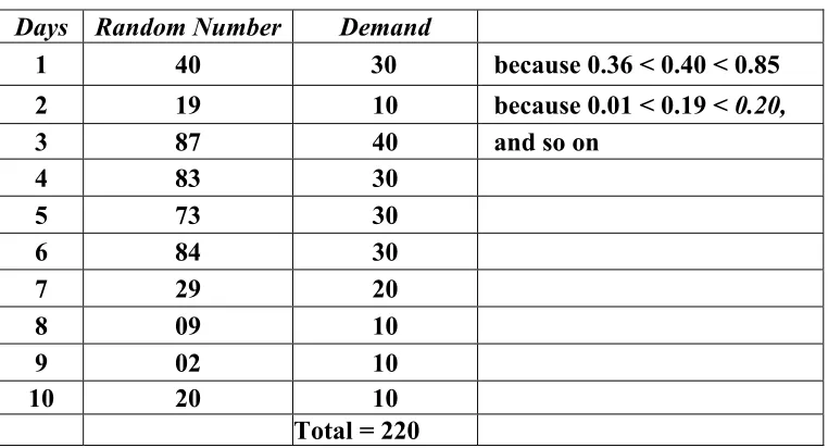
The simulation calculations for a period of 10 days are given in table below:
Table 3 : Simulation Experiment
Days Random Number Demand
1 40 30 because 0.36 < 0.40 < 0.85 2 19 10 because 0.01 < 0.19 < 0.20,
3 87 40 and so on
4 83 30
5 73 30
6 84 30
7 29 20
8 09 10
9 02 10
10 20 10
Expected demand = 220/1 0 = 22 units per day
Example 3
A bookstore wishes to carry a particular book in stock. Demand is probabilistic and replenishment of stock takes 2 days (i.e. if an order is placed on March 1, it will be delivered at the end of the day on March 3). The probabilities of demand are given below:
Demand (daily) : 0 1 2 3 4
Probability : 0.05 0.10 0.30 0.45 0.10
Each time an order is placed, the store incurs an ordering cost of Rs. 10 per order. The store also incurs a carrying cost of Re 0.05 per book per day. The inventory carrying cost is calculated on the basis of stock at: the end of each day. The manager of the bookstore wishes to compare two options for his inventory decision
A : Order 5 books when the inventory at the beginning of the day plus orders outstanding is less than 8 books.
B: Order 8 books when the inventory at the beginning of the day plus orders outstanding is less than 8.
Currently (beginning of 1st day) the store has a stock of 8 books plus 6 books ordered two days ago and expected to arrive next day. Using Monte Carlo simulation for 10 cycles, recommend which option the manager should choose.
The two digit random numbers are: 89, 34, 78, 63, 61, 81, 39, 16, 13, 73
Solution
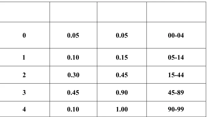
Using the daily demand distribution, we obtain a probability distribution as shown in Table 4 below
Table 4 Daily Demand Distribution
0 0.05 0.05 00-04
1 0.10 0.15 05-14
2 0.30 0.45 15-44
3 0.45 0.90 45-89
4 0.10 1.00 90-99
Given that stock in hand is of 8 books and stock on order is 5 books (expected next day)
Table 5 Option A
Random Number
Daily
Demand Stock in Closing Hand
Receipt Opening Stock in
Hand
Stock on Order
Order
Quantity Closing Stock
(1) (2) (3) (4)
(4)+(3)-(2)=(5) (6) (7) (8)
89 3 8 - 8-3=5 6 - 6
34 2 5 6 6+5-2=9 - - -
78 3 9 - 9-3=6 - 5 5
63 3 6 - 6-3=3 5 - 5
61 3 3 - 3-3=0 5 5 10
81 3 0 5 5-3=2 5 5 10
39 2 2 - 2-2=0 10 - 10
16 2 0 5 5-2=3 5 - 5
13 1 3 5 5 + 3 - 1= 7 0 5 5
73 3 7 - 7-3=4 5 - 5
Closing stock of 10 days is of 39 (= 5 + 9 + 6 + 3 + 2 + 3 + 7 + 4) books. Therefore, the holding cost at the rate of Re 0.5 per book per day is Rs. (39 x 0.5) = Rs. 19.5.
Total cost for 10 days = Ordering cost + Holding cost = Rs. (40 + 19.5) = Rs. 59.5.
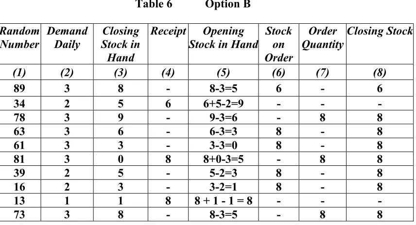
Table 6 Option B
Random Number Demand Daily Closing Stock in Hand Receipt Opening Stock in Hand
Stock on Order Order Quantity Closing Stock
(1) (2) (3) (4) (5) (6) (7) (8)
89 3 8 - 8-3=5 6 - 6
34 2 5 6 6+5-2=9 - - -
78 3 9 - 9-3=6 - 8 8
63 3 6 - 6-3=3 8 - 8
61 3 3 - 3-3=0 8 - 8
81 3 0 8 8+0-3=5 - 8 8
39 2 5 - 5-2=3 8 - 8
16 2 3 - 3-2=1 8 - 8
13 1 1 8 8 + 1 - 1 = 8 - - -
73 3 8 - 8-3=5 - 8 8
Since 8 books have been ordered three times as shown in Table 6, when the inventory of books at the beginning of the day plus orders outstanding is less than 8. Therefore, total ordering cost is : Rs. 30 (3 X 10)
Closing stock of 10 days is of 45 (=5+9+6+3+5+3+1+8+5) books. Therefore, holding cost, re. 0.5 per book is Rs. 22.50 (45 X 0.5)
Total cost for 10 days = Ordering Cost + Holding Cost + Rs. 52.20. Since option B has lower total cost than option A, therefore, manager should choose option B
Simulation of Queuing Problem
Example :
10 per hour, the bureau will have to have at least 2 people staffing the desk during the day. The bureau is open from 8am to 2pm each day. How much will it cost to staff the front desk?
From a single day's observation, we have gathered the following data (legacy):
In the first hour, 3 visitors arrive, the second hour 15 visitors arrive, then 4, 8, 12, and 8 respectively for the duration of the day.
Monte Carlo:
Hr. (variable) # Visitors Probability Cumulative Probability Random #'sIntervals of
8am-9am 3 3/50 = .06
9am-10am 15 15/50 = .30
10am-11am 4 .08
11am-12noon 8 .16
12noon-1pm 12 .24
1pm-2pm 8 .16
Total 50 1.0
In the above table, we set up the variables, the values for the variables (#visitors) and the probability of each value occurring.
Now we want to add the cumulative probabilities to the table:
Hr. (variable) # Visitors Probability Cumulative Probability
Intervals of Random #'s
8am-9am 3 3/50 = .06 .06
9am-10am 15 15/50 = .30 .36
10am-11am 4 .08 .44
11am-12noon 8 .16 .60
12noon-1pm 12 .24 .84
1pm-2pm 8 .16 1.0
Total 50 1.0 1.0
Hr. (variable) # Visitors Probability Cumulative Probability
Intervals of Random #'s
8am-9am 3 3/50 = .06 .06 00-05
9am-10am 15 15/50 = .30 .36 06-35
10am-11am 4 .08 .44 36-43
11am-12noon 8 .16 .60 44-59
12noon-1pm 12 .24 .84 60-83
1pm-2pm 8 .16 1.0 84-99
Total 50 1.0 1.0
We then determine how many trials we are going to run. Let's say we want to run 10 trials. We generate random numbers from our Random Number Table (given in last lesson) to run these trials.
Let's use Row 1 from the table to get our random numbers. When a random number is generated, we look to see where it falls relative to the random intervals established above. We then assign the value (# visitors) to :
Trial Random Generated Number
# of Visitors from Random Intervals
1 52 8
2 06 15
3 50 8
4 88 8
5 53 8
6 30 15
7 10 15
8 47 8
9 99 8
10 37 4
Total = 97
97/10 = 9.7
Based on this information, we do not need to staff another person at the front desk. Our total daily costs are:
(6hrs/day)*($6/hr) = $36/day
Similarly Monte Carlo Simulation is useful and can be applied for Investment Analysis, Maintenance Policies, Operational Gaming, and Systems Simulation.