Reconstructing the Nd oceanic cycle using a coupled dynamical – biogeochemical model

www.biogeosciences.net/6/2829/2009/

© Author(s) 2009. This work is distributed under the Creative Commons Attribution 3.0 License.

Biogeosciences

Reconstructing the Nd oceanic cycle using a coupled dynamical –

biogeochemical model

T. Arsouze1,2,*, J.-C. Dutay1, F. Lacan2, and C. Jeandel2

1_{Laboratoire des Sciences du Climat et de l’Environnement (LSCE), IPSL, CEA/UVSQ/CNRS, Orme des Merisiers,}

Gif-Sur-Yvette, Bat 712, 91191 Gif sur Yvette cedex, France

2_{Laboratoire d’Etudes en G´eophysique et Oc´eanographie Spatiale (LEGOS), UPS/CNES/CNRS/ IRD, Observatoire}

Midi-Pyr´en´ees, 14 av. E. Belin, 31400 Toulouse, France

*_{now at: Lamont-Doherty Earth Observatory (LDEO), P.O. Box 1000 61 Route 9W, Palisades, NY 10964-1000, USA}

Received: 11 May 2009 – Published in Biogeosciences Discuss.: 10 June 2009

Revised: 9 November 2009 – Accepted: 24 November 2009 – Published: 4 December 2009

Abstract. The decoupled behaviour observed between Nd

isotopic composition (Nd IC, also referred asεNd) and Nd

concentration cycles has led to the notion of a “Nd para-dox”. WhileεNdbehaves in a quasi-conservative way in the

open ocean, leading to its broad use as a water-mass tracer, Nd concentration displays vertical profiles that increase with depth, together with a deep-water enrichment along the global thermohaline circulation. This non-conservative be-haviour is typical of nutrients affected by scavenging in sur-face waters and remineralisation at depth. In addition, re-cent studies suggest the only way to reconcile both concen-tration and Nd IC oceanic budgets, is to invoke a “Bound-ary Exchange” process (BE, defined as the co-occurrence of transfer of elements from the margin to the sea with re-moval of elements from the sea by Boundary Scavenging) as a source-sink term. However, these studies do not sim-ulate the input/output fluxes of Nd to the ocean, and there-fore prevents from crucial information that limits our un-derstanding of Nd decoupling. To investigate this paradox on a global scale, this study uses for the first time a fully prognostic coupled dynamical/biogeochemical model with an explicit representation of Nd sources and sinks to simu-late the Nd oceanic cycle. Sources considered include dis-solved river fluxes, atmospheric dusts and margin sediment re-dissolution. Sinks are scavenging by settling particles. This model simulates the global features of the Nd oceanic cycle well, and produces a realistic distribution of Nd con-centration (correct order of magnitude, increase with depth and along the conveyor belt, 65% of the simulated values fit in the±10 pmol/kg envelop when compared to the data)

Correspondence to: T. Arsouze

([email protected])

and isotopic composition (inter-basin gradient, characteriza-tion of the main water-masses, more than 70% of the simu-lated values fit in the±3εNdenvelop when compared to the

data), though a slight overestimation of Nd concentrations in the deep Pacific Ocean may reveal an underestimation of the particle fields by the biogeochemical model. Our results indicate 1) vertical cycling (scavenging/remineralisation) is absolutely necessary to simulate both concentration andεNd,

and 2) BE is the dominant Nd source to the ocean. The estimated BE flux (1.1×1010g(Nd)/yr) is much higher than both dissolved river discharge (2.6×108g(Nd)/yr) and atmo-spheric inputs (1.0×108g(Nd)/yr) that both play negligible role in the water column but are necessary to reconcile Nd IC in surface and subsurface waters. This leads to a new cal-culated residence time of 360 yrs for Nd in the ocean. The BE flux requires the dissolution of 3 to 5% of the annual flux of continental weathering deposited via the solid river dis-charge to the continental margin.

1 Introduction

Variations in neodymium isotopic composition (hereafter re-ferred as Nd IC1) observed within the ocean reflect influ-ences from both lithogenic inputs of the element (whose IC varies as a function of age and geological composition of

1_{By convenience, we preferentially use}

the εNd parameter defined as: εNd =

143_Nd.

144_Nd

sample

,

143_Nd.

144_Nd

CHUR

−1

!

· 104,

where

143_Nd.

144_Nd

CHUR

the continent, Jeandel et al., 2007) and the subsequent re-distribution by oceanic circulation.εNddata show that these

variations are closely linked to water mass distribution at depth, and that far from any continental sources, Nd IC be-haves quasi-conservatively (Piepgras and Wasserburg, 1982; Jeandel, 1993; von Blanckenburg, 1999; Goldstein and Hem-ming, 2003). Hence, the main water masses display charac-teristicεNd values (e.g. NADW: εNd≈ −13.5, AAIW and

AABW: εNd≈ −8). This water mass tracer property has

been recently explored in the modern ocean, by measuring dissolved Nd IC and concentrations (Jeandel, 1993; Piep-gras and Wasserburg, 1980; PiepPiep-gras and Wasserburg, 1982, 1987; Shimizu et al., 1994; Lacan 2004), but has also been used for reconstructing past ocean circulation from measure-ments in the authigenic fraction of sedimeasure-ments (Rutberg et al., 2000; Piotrowski et al., 2004, 2005; Gutjahr et al., 2008). The water mass tracer property ofεNdis commonly accepted,

however our understanding of the complete Nd oceanic cycle is far from sufficient to allow a reliable use of this proxy as a paleocirculation tracer (Arsouze et al., 2008). In particu-lar, the nature and the relative importance of the different Nd sources and sinks, and the dissolved/particulate interactions within the water column remain unconstrained.

Previous studies show a decoupling behaviour between Nd concentration and its IC in the open ocean (Bertram and El-derfield, 1993; Jeandel et al., 1995; Tachikawa et al., 1999, 2003; Lacan and Jeandel, 2001). This feature has been named the “Nd paradox” (Tachikawa et al., 2003; Goldstein and Hemming, 2003; Lacan and Jeandel, 2005), and results in different properties characterizing the Nd concentration and its IC distribution in the dissolved phase. Vertical pro-files of Nd concentration are similar to that of all Rare Earth Elements (excluding Ce), showing low values in surface wa-ters which increase with depth, suggesting the influence of vertical cycling (i.e. the element is scavenged at the surface, sinks with the particles, and is subsequently remineralized at depth). Furthermore, Nd concentrations increase along the thermohaline circulation, which is a typical distribution for nutrients like silicate (Elderfield, 1988), whose characteristic residence time is on the order of∼2×104 years (Broecker and Peng, 1982). In contrast, pronouncedεNdvariations

be-tween each oceanic basin indicate that the Nd residence time is shorter than the global oceanic mixing time estimated to

∼103years (Broecker and Peng, 1982). The conservativity ofεNdwithin the major oceanic water masses suggests at first

sight thatεNdmay vary in the open ocean only by water-mass

mixing, excluding vertical cycling.

It has been demonstrated that Nd oceanic budgets that con-sider only dissolved river and atmospheric dust inputs fail to balance both concentration and Nd IC (Bertram and El-derfield, 1993; Tachikawa et al., 2003; van de Flierdt et al., 2004). Other sources have been suggested in order to rec-oncile the budget of both quantities, like submarine ground-waters (Johannesson and Burdige, 2007) or input from con-tinental margin inputs (Tachikawa et al., 2003) subsequently

leading to the notion of “Boundary Exchange” (BE, strong interactions between continental margin and water masses by co-occurrence of sediment dissolution and Boundary Scav-enging, Lacan and Jeandel, 2005). This last process has the advantage of including both a source (Boundary Source) and a sink (Boundary Scavenging) for the element, affecting the IC without changing the observed concentration when both fluxes are similar.

Resolving the “Nd Paradox” hence resides in 1) finding the vertical processes responsible for both Nd concentration increase with depth and the Nd IC conservative property in the water column, and 2) constraining the missing source which may explain the important observed Nd IC gradient observed along the thermohaline circulation together with the relatively moderated increase of Nd concentrations.

Recent modelling of oceanicεNd, schematically presented

in Fig. 1, has helped to improve our understanding of the Nd oceanic cycle. Arsouze et al. (2007, Fig. 1a), taking into account only BE as a source/sink term, simulated a realis-tic globalεNddistribution, suggesting that this process plays

a major role in the oceanic cycle of the element. However, this first approach was based on the simulation of the Nd IC only (the Nd concentration being considered constant), us-ing a simple relaxus-ing term parameterization for the BE pro-cess. Given that no source flux is explicitly considered in this method, the authors could not address the “Nd paradox” and quantify the processes acting in the oceanic Nd cycle. Jones et al. (2008, Fig. 1b) considered no external sources, but pre-scribed surface Nd IC with observations, to conclude thatεNd

behaves conservatively in the ocean (changing only by water mass mixing). However they needed to invoke an input to the deep North Pacific, which could represent an input directly to the deep ocean (e.g. by boundary exchange), or vertical cy-cling. We underline here that prescribingεNdat the surface

must be considered as an implicit source of Nd, in contradic-tion to the conclusion of these authors upon the role of mix-ing. Lastly, Siddall et al. (2008, Fig. 1c) have modelled ex-plicitly both Nd concentration and IC using a reversible scav-enging model to test the influence of vertical cycling in the oceanic distribution of this element. These authors suggest that both scavenging and remineralisation processes are im-portant for explaining Nd concentration and IC profiles, con-sistent with the conclusions of Bertram and Elderfield (1993) and Tachikawa et al. (1999, 2003). If the results of Siddall et al. (2008) provide important implications for solving the “Nd paradox”, the authors can not in return estimate the dif-ferent fluxes involved in the Nd cycle. Indeed, this study by Siddall et al. (2008) is prescribing Nd concentration and

εNdto observations in surface waters, and leaves the detailed

Atmospheric dusts Dissolve fluvial material

3000m

Sediment remobilization

Sedimentation

Reversible Scavenging

Sedimentation

Reversible Scavenging

3000m Continental margin

Boundary Exchange

A)

C)

B)

D) Modelingε_Nd

Modelingε

Ndand [Nd]

Prescribed by data Process studied

Relaxing term

Arsouze et al. 2007

Siddall et al., 2008 This study

Jones et al., 2008

Continental margin

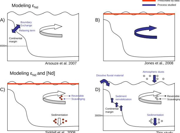
Fig. 1. Summary of the main published Nd oceanic modelling efforts using an OGCM. In each case, the different processes explicitly

simulated are represented. Arrows and legends in blue underline the processes specifically studied, while red components refer to parameters prescribed by the data. (A) Arsouze et al. (2007), modelling only Nd IC, focused on the role of Boundary Exchange using a relaxing term and defined on the first 3000 m of the continental margin: this work highlighted the importance of this process in the element’s global cycle.

(B) Jones et al. (2008), prescribing a surfaceεNdvalue estimated by the data suggested that Nd IC distribution can simply be explained by

water mass mixing, except in the North Pacific region, where some external radiogenic inputs are required. (C) Using prescribed surfaceεNd

and Nd concentration, as well as particle fields determined by satellite observations and then interpolated within the water column, Siddall et al. (2008) showed the major role of vertical cycling (reversible scavenging process) to reproduce bothεNdand Nd concentration oceanic

distribution. (D) In this study, besides confirming, as in Siddall et al. (2008), the role of vertical cycling in Nd oceanic distribution, we aimed to determine and quantify the different sources involved in the Nd oceanic cycle. The Boundary Exchange process is implicitly taken into account via sediment redissolution along the continental margins (source term) as well as by particle sedimentation (sink term).

al., 2008) and Nd concentration, as well as particle distri-bution (imposed by satellite data and then extrapolated into the water column, Siddall et al., 2008) limits any potential paleo-application.

This study continues the modelling work initiated by Tachikawa et al. (2003), Arsouze et al. (2007) and Siddall et al. (2008) using a coupled dynamical (Ocean Global Circula-tion Model, that generates dynamical fields)/biogeochemical (dedicated to carbon cycle and ecosystems studies, that sim-ulates particle fields in the ocean) model. The vertical cy-cling is simulated using a reversible scavenging model devel-oped for the simulation of trace elements with this coupled model (Dutay et al., 2009). Although these authors identi-fied some limitations of this coupled model for geochemical tracer modelling, as we will see hereafter, our approach is dictated by the need for collaboration with carbon cycling modellers to initiate further studies aimed at developing the biogeochemical model. Such developments may lead to mu-tual advance for both carbon cycle and geochemical (Pa, Th,

δ13C, Nd, etc. . . ) modelling (Dutay et al., 2009), and also to a significant improvement on our understanding of the ele-ment oceanic cycles in the long term, mostly in the context of the increasing database that will result from the

interna-tional GEOTRACES effort (GEOTRACES, 2005). Also, this model is fully prognostic so that it can be easily used for pa-leo applications or even future climate scenarios.

We explicitly represent and quantify the different sources implied in the oceanic cycle of the element (Fig. 1d). This allows investigation from an independent approach 1) if the Boundary Source could globally represent the primordial flux of the tracer into the ocean, as suggested by Arsouze et al. (2007), and 2) if the Boundary Source and Boundary Scanvenging fluxes of the BE process can be associated with the “missing flux” proposed by Tachikawa et al. (2003) in order to balance the Nd oceanic budget.

2 Modelling the Nd oceanic cycle

2.1 The dynamical model NEMO-OPA

The dynamical model used is the NEMO-OPA model (IPSL/LOCEAN, Madec, 2006). It includes the sea-ice model LIM (Louvain-La Neuve, Fichefet and Maqueda, 1997), in its low-resolution configuration ORCA2. The defi-nition of the mesh is based on a 2◦×2◦×cos (latitude) MER-CATOR grid, with poles defined on the continents so as to get rid of singularities near the North Pole. Meridional resolu-tion increases to 0.5◦near the equator, in order to account for the specific local dynamics. Vertical resolution varies with depth, from 10 m at the surface (12 levels included in the first 125 m) to 500 m at the bottom (31 levels in total). The model is forced at the surface by heat and freshwater fluxes obtained from bulk formulae and ERS satellite data from the tropics, and NCEP/NCAR data from polar regions. Surface salinity is readjusted every 40 days to monthly WA01 data to prevent model drift (Timmermann et al., 2005). The Tur-bulent Kinetic Energy closure is applied to the mixing layer (Blanke and Delecluse, 1993), and subscale physics is pa-rameterized using the Gent and McWilliams scheme (1990). The same model, in similar configurations, has previously been used for other geochemical tracer simulations (Dutay et al., 2002, 2004, 2009; Doney et al., 2004; Arsouze et al., 2007). Despite classical shortcomings of low resolution models (boundary currents too weak, crude representation of sinking of dense water during deep water masses formation), this model satisfyingly simulates the main structures of the global thermohaline circulation.

2.2 The biogeochemical model PISCES

The biogeochemical model PISCES developed for carbon cycle modelling was coupled to NEMO. It is a prognostic ecosystem and oceanic carbon cycle model, based on the Hamburg Model of Carbon Cycle version 5 (HAMOCC5, Aumont et al., 2003), that represents the biogeochemical cy-cles of carbon, oxygen, and five nutrients of primary pro-duction (phosphates, nitrates, silicates, ammonium and iron). Redfield ratios are set constant, and are based on phytoplank-ton growth limited by nutrient availability (Monod, 1942).

The model features two classes of phytoplankton (nanophytoplankton and diatoms), and two classes of zoo-plankton (microzoozoo-plankton and mesozoozoo-plankton), as well as three non-living components, including Dissolved Organic Carbon (DOC), small and large particles. Small particles (particles between 2 and 100µm in size) have a sinking ve-locity of 3 m/day (determined using the relationship between particle size and the sinking velocity established by Kriest, 2002), and consist of Particulate Organic Carbon (POCs). Large particles include Particulate Organic Carbon with a diameter larger than 100µm (POCb), biogenic silica (BSi), calcite (CaCO3)and lithogenic particles (atmospheric dust),

sinking with a velocity varying from 50 m/day at the surface to 300 m/day at depth. The two classes of POC interact via the processes of aggregation/disaggregation. Also a reminer-alization process depending on temperature (with aQ10 of

about 1.9) is represented between POCb and POCs, and be-tween POCs and DOC (Aumont and Bopp, 2006). The refer-ence of 100µm used to differentiate small and large carbon-ate particles (POCs and POCb, respectively) does not corre-spond to the definition used by experimentalists, who usually refer to large particles as particles collected in traps or by large volume filtration and has having a diameter larger than 50µm. This being so, the size range of particles trapped re-mains unknown. In addition, the particles observed by the Underwater Video Profilers (UVP, Gorsky, 2000) have a di-ameter larger than 100µm meaning the same limit as pre-scribed in the model.

A more detailed description of the model, as well as the equations used, are available as supplementary material of Aumont and Bopp (2006).

An evaluation of the particle fields generated by the PISCES model with available data collected by particle traps, satellite observations and estimations, was performed by Gehlen et al. (2006) and Dutay et al. (2009). The small par-ticle pool represents the main parpar-ticle stock at the surface (at least one order of magnitude higher than the large particle concentration). The simulated small particle concentrations in surface waters are in agreement with observations, mostly in regions of high productivity (coastal upwellings, Equato-rial Pacific, Austral Ocean). In contrast, PISCES generates exaggerated vertical variations of the small particle distribu-tions at depth in the water column leading to small particles concentrations that are too low, due to remineralization and aggregation processes. This POCs vertical gradient largely overestimates the available observations (only a factor of 50 between surface and depth, compared to a factor of 1000 for the model). In contrast, the few CaCO3and BSi vertical

pro-files observed in the water column are successfully replicated by the model (Dutay et al., 2009).

2.3 The reversible scavenging model

Considering Nd dissolved concentrations (Ndd)and Nd

particulate concentrations (concentration of Nd by unity of particle mass, Ndp), the equilibrium partition coefficientK

is defined as:

K= Ndp

NddCp

(1) whereCpis the mass of particles per mass of water. This

co-efficientK is defined for each type of particles represented in the model: small (POCs) and big (POCb) Particulate Or-ganic Carbon, Biogenic Silica (BSi), calcite (CaCO3) and

lithogenic atmospheric dust (litho).

We model the two 143Nd and 144Nd isotopes indepen-dently and calculate εNd and Nd concentration afterward.

Observations do not suggest any fractionation between

143_{Nd and}144_{Nd dissolved, colloidal and particulate phases}

(Dahlqvist, 2005), as they are two isotopes of the same el-ement, and their masses are quite similar. Partition coeffi-cients (K) are thus assumed as being identical for the two isotopes for each particle type.

In the model, we transport for both143Nd and144Nd trac-ers the total concentration (NdT), defined as the sum of

dis-solved concentration (Ndd), small (POCs: Ndps) and big

(POCb, BSi, CaCO, litho: Ndpg) particulate concentration:

NdT =Ndps+Ndpg+Ndd (2)

Applying Eq. (1) to the particulate pools to express total con-centration as a function of dissolved Nd concon-centration, we obtain:

NdT =(KPOCs∗CPOCs+KPOCb∗CPOCb+KBSi∗CBSi (3)

+KCaCO3∗CCaCO3+Klitho∗Clitho+1

∗Ndd

that leads to:

Ndps= (4)

KPOCsCPOCs

KPOCs∗CPOCs+KPOCb∗CPOCb+KBSi∗CBSi+KCaCO3∗CCaCO3+Klitho∗Clitho+1

∗N dT

Ndpb= (5)

KPOCb∗CPOCb+KBSi∗CBSi+KCaCO3∗CCaCO3+Klitho∗Clitho

KPOCs∗CPOCs+KPOCb∗CPOCb+KBSi∗CBSi+KCaCO3∗CCaCO3+Klitho∗Clitho+1

∗N dT

This allows Nd concentrations in small and big particles to be defined a posteriori as a function of partition coefficients and total Nd concentration. The main advantage of this method is that we simulate explicitly the total concentration of the two isotopes (two tracers143NdT and144NdT)rather than

con-centration in every phase (dissolved, small particles and all big particles, meaning 12 tracers), which implies a substan-tial gain of computational cost.

The evolution of the total concentration of the tracer is equal to the sum of all sources (A), influence of vertical cy-cling (B) and physical transport by advection and diffusion (C). The conservation equation of the tracer can therefore be written:

∂NdT

∂t =S (| Nd{zT})

(A)

(6)

−∂(wsNdps)

∂z −

∂(wbNdpb)

∂z

| {z }

(B)

−U· ∇NdT+ ∇ ·(k∇NdT)

| {z }

(C)

where S(NdT)is the Source term of the tracer (cf. Sect. 2.4).

The vertical cycling represents the scavenging of Nd by the particles (ws andwbare the sinking velocities of small and

big particles, respectively). The simulations are performed “off-line” using pre-calculated dynamical: velocity (U )and mixing coefficient (k), and particle (POCs, POCb, BSi, and CaCO3)distributions in order to reduce computational costs,

which allows us to perform some sensitivity tests.

2.4 Description of Nd sources and sink

One of our main objectives is to study the relative influence of the different sources of Nd to the ocean. We therefore explicitly represent the different source of Nd in the ocean in our simulations.

The source of the BE process (Boundary Source) is as-sumed to be the dissolution of a small percentage of the sed-iments deposited along the continental margin. We spec-ify this source in the model by imposing an input flux on each continental margin grid point of the model between 0 and 3000 m (Boillot and Coulon, 1998). This Nd Boundary Source is written as:

S(NdT)sed=

Z

S

Fsed∗maskmar∗f (z) (7)

whereFsedis the source flux of sedimentary Nd to the ocean

(in g(Nd)/m2/yr). Sediment flux is assumed here as geo-graphically constant. This hypothesis may be not verified in the ocean and disparities could play an important role on a global scale. However, considering the lack of knowledge of the processes acting on this source, it seems reasonable to set it as constant as a first approximation. Fsed is then

determined for both143Nd and144Nd isotopes by multiply-ing this sediment flux to the concentration along the margin. This is set up viaεNddefinition and Nd isotopes abundances,

using Nd concentration and εNd maps along the

continen-tal margins (Fig. 2a and b), both generated in a similar way by interpolation of a recent data compilation (Jeandel et al., 2007). We use the high-resolution ETOPO-2 bathymetry to calculate, for each grid cell of the model, the percentage of continental margin surface within the cell with respect to the surface of the cell (maskmar). This determines, for a

180°W 120°W 60°W 0° 60°E 120°E 180°E 60°N

0°

60°S

180°W 120°W 60°W 0° 60°E 120°E 180°E 60°N

0°

60°S

180°W 120°W 60°W 0° 60°E 120°E 180°E 60°N

0°

60°S

180°W 120°W 60°W 0° 60°E 120°E 180°E 60°N

0°

60°S

180°W 120°W 60°W 0° 60°E 120°E 180°E 60°N

0°

60°S

180°W 120°W 60°W 0° 60°E 120°E 180°E 60°N

0°

60°S A)

C)

E)

B)

D)

F) Nd IC of margins (in εNd)

Nd IC of rivers (in εNd)

Nd IC of atmospheric dusts (in εNd)

Nd concentration of margins (in pmol/kg)

Nd concentration of rivers (in μg/g)

River runoff (in 1015_g/yr)

15 10 5 0 -5 -10 -15 -20 -25 -30 -35 -40

10 5 0 -5 -10 -15 -20 -25

0 -4

-12 -16 -20 -24 -28 -8

55 50 45 40 35 30 25 20 15 10 5 0 60

200 100 90 80 70 60 50 40 30 20 10 0

800 100₉₀ 80 70 60 50 40 30 20 109 87 65 43 21 0

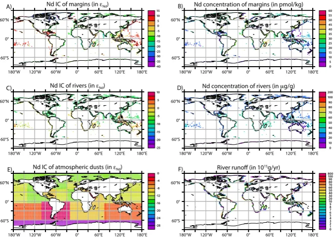
Fig. 2. Input maps applied to the model. (A)εNd map along the continental margin determined by Jeandel et al. (2007). This input is

applied to the sedimentary remobilization sourceFsed. (B) Nd concentration map along continental margin (inµg/g) determined by Jeandel

et al. (2007). This input is also applied to the sedimentary remobilization sourceFsed. (C)εNdmap of river runoff given by Goldstein and

Jacobsen (1987). (D) Nd concentration of river runoff (in ng/g) Goldstein and Jacobsen (1987); scale is non linear. (E) InterpolatedεNd

map of atmospheric dust (Grousset et al., 1988; Grousset et al., 1998; Jeandel et al., 2007). Dust particle fields are provided by Tegen and Fung (1995), and Nd concentration is set constant to 20µg/g. (F) Runoff map prescribed by NEMO OGCM (in 1015g/an). Scale is non linear.

layer depth. Also, we multiplyFsed by a vertical function

equal to 1 in the first 1000 m, then exponentially decreasing at depth (f (z)). This vertical variation has been applied in accordance with iron modelling (Aumont and Bopp, 2006) and previousεNd modelling studies (Arsouze et al., 2007),

because we suppose that the sediment dissolution is more important in surface waters than at depth (at the surface, dy-namic activity is more vigorous, and biological processes are more important). The only available global estimation of the Nd Boundary Source flux is the “missing flux” calculated by Tachikawa et al. (2003). We therefore use their value of 8.0×109g(Nd)/yr as a reference for our simulations.

In addition to Boundary Sources, dissolved river discharge (defined on continental margin points only) and atmospheric dust deposit are taken into account as Nd inputs in surface waters (first vertical level).

S(NdT)surf=

Z

S

Fsurf (8)

whereFsurfis the Nd flux of these two sources to the ocean

(in g(Nd)/m2/yr).

For dissolved river discharge we use the climatological runoff applied to the dynamical model (Fig. 2f). Nd IC (Fig. 2c) and concentrations (Fig. 2d) in river inputs are es-timated using the compilation of data provided by Goldstein

and Jacobsen (1987). Using the runoff estimation provided by the NEMO model, and a subtraction of 70% of material in the estuaries (Sholkovitz, 1993; Elderfield et al., 1990; Nozaki and Zhang, 1995), we obtain a Nd dissolved flux from rivers of 2.6×108g(Nd)/yr (Table 1). This value is lower, but the same order of magnitude, than the flux used by Tachikawa et al. (2003), equal to 5×108g(Nd)/yr.

Atmospheric dust flux is determined using monthly maps provided by Tegen and Fung (1995), in agreement with the method used for the PISCES model for nutrients (Aumont and Bopp, 2006). Nd IC of this source has been established using available data (Grousset et al., 1988, 1998). How-ever, in the areas where no data were available, theεNd of

the dust is determined according to theεNdvalue for the

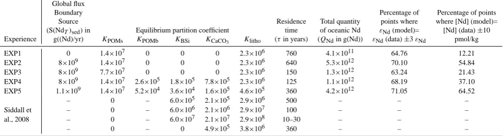
Table 1. Main characteristics of equilibrium partition coefficients and source fluxes for each experiment. Residence time of Nd in the ocean

is calculated using the sum of flux (source or sink) and the total quantity of Nd simulated in the ocean:τ=QNd/(S(NdT)sed+S(NdT)surf).

Also, for comparison purpose, values of equilibrium partition coefficient and residence time from Siddall et al. (2008) have been added.

Global flux

Boundary Percentage of Percentage of points

Source Residence Total quantity points where where [Nd] (model)=

(S(NdT)sed)in Equilibrium partition coefficient time of oceanic Nd εNd(model)= [Nd] (data)±10

Experience g((Nd)/yr) KPOMs KPOMb KBSi KCaCO3 Klitho (τin years) (QNdin g(Nd)) εNd(data)±3εNd pmol/kg

EXP1 0 1.4×107 _{0 0 0 2.3×10}6 _{760 4.1×10}11 _{64.76 12.21}

EXP2 8×109 _1.4×107 _{0 0 0 2.3×10}6 _{640 5.3×10}12 _{70.10 54.84}

EXP3 8×109 7.7×107 0 0 0 2.3×106 150 1.3×1012 63.24 21.43

EXP4 8×109 1.4×107 2.6×105 1.8×105 7.8×105 2.3×106 125 1.1×1012 68.19 37.10

EXP5 1.1×109 1.4×107 5.2×104 3.6×104 1.6×105 4.6×105 360 4.2×1012 71.05 64.52

– 0 – 6.0×105 2.1×105 2.9×106 500 – – –

Siddall et – 0 – 6.0×106 2.1×106 2.9×107 100 – – –

al., 2008 – 0 – 6.0×107 2.1×107 2.9×108 10–30 – – –

– 0 – 0 4.9×105 3.8×106 360 – – –

Zhang et al. (2008) reconsidered all this data and estimated that this percentage does not exceed 10%. We finally obtain a flux of 1×108g(Nd)/yr (Table 1). Still, this value is lower than Tachikawa et al. (2003) who considered the earlier Duce et al. (1991) atmospheric dust deposit estimation, leading to a flux of 5×108g(Nd)/yr. Additional sensitivity tests on both dissolution rate ratios for atmospheric dusts and Nd dissolved river discharge (not shown here) do not significantly change the results and conclusions presented here.

The re-dissolution of solid material deposited by rivers at estuary mouths is potentially a source of great importance (Sholkovitz, 1993; von Blanckenburg et al., 1996). However, this source is implicitly taken into account via the Bound-ary Source (Fsed), as we consider that all material deposited

along the continental margin is made available for sediment re dissolution.

To balance the budget of Nd in the ocean, the only Nd sink considered is the burying of particles in the sediment at the bottom of the water column, i.e. scavenging. The particle-associated neodymium sinking at the deepest level thus leaves the model. Simulations are run until 143Nd and144Nd oceanic concentrations reach an equilibrium state, which is when the sink balances global sources.

3 Simulation description

Currently the available observations of Nd concentrations in particulate phases, which allow constraint of the equilib-rium partition coefficients (K) are scarce. In addition, the pool of particles generated by the PISCES model is bio-genic, whereas data suggest that particulate Nd, is mainly adsorbed on the hydroxide phases coating the biogenic par-ticles (Sholkovitz et al., 1994). Nd concentrations in iron or manganese hydroxides are at least an order of magnitude

higher than those observed for biogenic particles (Bayon et al., 2004). The fact that PISCES does not take into ac-count these particles might be critical to simulate realistic Nd dissolved-particulate interactions. Nevertheless, observa-tions in the Atlantic and Austral basins, give an estimation of Ndp/Nddvalues between 0.05 and 0.1 (Jeandel et al., 1995;

Tachikawa et al., 1997; Zhang et al., 2008).

Using the same model for their231Pa and 230Th simula-tions, Dutay et al. (2009) have shown the necessity to im-pose a variation of the partition coefficient as a function of particle stock, in order to simulate realistic vertical profiles for both the dissolved and particulate phases. In addition, the scavenging of these tracers had to be controlled by the small particle pool, and thus the value of their partition coef-ficients with this pool had to be greater than those applied to the big particles. We adopt this approach for our Nd simu-lation and therefore set equilibrium partition coefficients for the big particle pools lower than those for the small particle pool.

Lastly, contrary to 231Pa and 230Th isotopes, for which scavenging coefficients can vary from several orders of mag-nitude depending on the particulate pool (Dutay et al., 2009), there is no current evidence from Nd data that preferential scavenging occurs when biogenic silica or carbonate dom-inate the particle pool. Thus we only differentiated small and big particles. The same equilibrium partition coeffi-cient value is taken for each pool of big particles, consider-ing their global averaged concentrations (POCb, BSi, CaCO3

and litho). Characteristics of sensitivity tests performed on K values performed are summarized in Table 1 (EXP3, EXP4 and EXP5).

and lithogenic particles are taken into account to simulate the vertical cycle. We take KPOMs=1.4×107 and Klitho=

2.3×106 that correspond to NdP/Ndd=0.001 and 1×10−4

respectively, andK=0 for remaining particle pools (POMb, CaCO3, BSi, cf. Table 1). Although these values are much

lower than the available data (Tachikawa et al., 1997), they are taken close to the same order of magnitude as in Siddall et al. (2008), and normalized to unit NdP/Nddvalue.

In a second experiment (EXP2), we consider the same con-figuration as the first simulation, but we added the sediment remobilization source (Boundary Source).

EXP3 and EXP4 test the sensitivity of the vertical cycling, considering the same sources of Nd as those considered in EXP2. For the third experiment (EXP3), we enhanced the small particle role relative to EXP2 by increasing the value of the equilibrium partition coefficient on small particles to

KPOMs=7.7×107 (which is equivalent to NdP/Ndd=0.005).

In the fourth experiment (EXP4) we have inserted the big particles (POMb, CaCO3, BSi) that were neglected in the

first three experiments, the other equilibrium partition coef-ficients being identical to those of EXP2. The equilibrium partition coefficient value for big particles in EXP4 is set two orders of magnitude lower than for small particles, consider-ing their respective concentrations in the PISCES model, i.e.

KPOCb=2.6×104,KBSi=1.8×104andKCaCO3=7.8×10

4_that

correspond to Ndp/Ndd=1×10−5(Table 1).

Finally, in the last experiment (EXP5) we optimized the characteristics of both our dynamical and biogeochemical models according to the information gained through the pre-vious tests, in order to produce the most realistic simula-tion. BE flux is adjusted to F(NdT)sed=1.1×1010g(Nd)/yr

and equilibrium partition coefficients are slightly reduced compared to EXP4 for POMb, CaCO3, BSi and litho, and

un-changed for the small particles (Table 1). Depending on the estimations, only between 3 and 5% (Milliman and Syvitski, 1992) dissolution of Nd material is required to explain our total Boundary Source flux S(NdT)sed=1.1×1010g(Nd)/yr.

4 Results

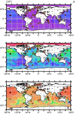
For each experiment, both Nd IC and concentration are shown along meridional sections in the Pacific Ocean (av-eraged zonally between 120◦W and 160◦W) and along the western boundary of the Atlantic Ocean (Figs. 3 and 5), where the water massεNdhave been characterized. Figures 4

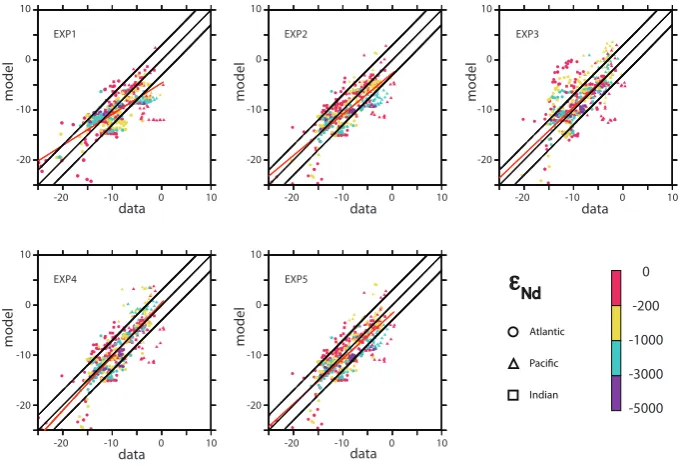
and 6 are scatter plots showing model and observations and Figs. 7, 8, 9 and 10 display horizontal maps ofεNdin surface

(0–200 m) and at depth (2500–4000 m), and Nd concentra-tion averaged over the same depth ranges, respectively.

The first experiment (EXP1) produces a satisfactoryεNd

distribution in surface waters (Fig. 7), but is much too ho-mogeneous in the deep ocean (Figs. 3, 5 and 8), particularly in the Atlantic basin, where the signature of the main wa-ter masses (NADW, AAIW, AABW) are not correctly

sim-ulated. Moreover, the Nd concentrations are at least an or-der of magnitude too low compared to the observations (av-erage global value of [Nd] (model)=2.3 pmol(Nd)/kg, [Nd] (data)=21.5 pmol(Nd)/kg and only 12% of modelled Nd con-centrations fit into the±10 pmol/kg envelop when compared to the data, Fig. 5 and Table 1).

In the second experiment (EXP2, BE added), simulated

εNdvalues in surface waters are still in agreement with the

observed data, and its distribution in the deep Atlantic Ocean is closer to the observed data. Indeed, the water masses in this basin are now simulated with very realisticεNd values

(Fig. 3): AABW (εNd (model) ∼= −10, εNd (data) ∼= −8)

but also AAIW (εNd (model) ∼= −8, εNd (data)∼= −8) and

NADW (εNd(model)∼= −13,εNd (data)∼= −13).

Contrast-ingly, simulated εNd values in the deep Pacific Ocean are

still much too negative when compared with the observa-tions (εNd(model) ∼= −10,εNd (data) =−4, Fig. 8), hence

producing anεNdinter-basin gradient wich is much too

ho-mogeneous. As a consequence, the simulated Nd concen-trations (Figs. 5 and 6) display values in the global ocean which are too high (average global value of [Nd] (model) = 35.7 pmol(Nd)/kg). The Nd vertical profiles are too pro-nounced, with realistic values at intermediate depth in both the Atlantic and Pacific basins, but concentrations are too low in surface waters, and too high at depth, particularly in the Pacific basin (Figs. 5 and 6). It should also be noted that this simulation produces a realistic increase of concentrations along the thermohaline circulation, in agreement with the ob-servations.

Increasing the value of the equilibrium partition coeffi-cient on small particles in the third experiment (EXP3) leads to a strengthening of the vertical cycling effect on simu-lated εNd and Nd concentrations. It results in an

undesir-able vanishing of NADW isotopic signature along its path-way in the Atlantic Ocean (Fig. 3). However it improves the

εNddistribution in the deep Pacific Ocean where values

be-comes more radiogenic (Fig. 8), but also leads to unrealistic high values at intermediate depths. Increasing vertical cy-cling enhances the sedimentation process (sink of Nd), and excessively reduces the simulated Nd concentrations ([Nd] (model) = 6.8 pmol(Nd)/kg and only 21% fit into the [Nd] (model) = [Nd] (data)±10 pmol/kg envelop, Fig. 5 and Ta-ble 1). The decrease of total Nd concentration with a constant source flux leads to a reduction of the residence timeτ (de-fined asτ=(F(Nd)surf+F(Nd)sed)/NdT)from∼700 years in

EXP1 and 2 to 150 years in EXP3 (Table 1).

Taking into account the influence of fast sinking biogenic big particles (POMb, CaCO3, bSi; EXP4) yields results close

1000

2000

5000 4000 3000

1000

2000

5000 4000 3000

PAC 120W - 160W

Western ATL section

1000

4000 3000 2000

5000 -14 -12 -10 -8

3 3

3

1000

4000 3000 2000

5000 1 -14 -10 -6 -2

1

1

1000

4000 3000 2000

5000 -14 -10 2-6 -2

2

2

1000

4000 3000 2000

5000 -18 -164-14 -12

4 4

1000

4000 3000 2000

5000 5

5

-14 -12 -10 -8 1000

4000 3000 2000

5000 -10 -6 3 -2 2

3

2

2 2

1000

4000 3000 2000

5000 -14 -10 -6 -2

1

!" 1

Data

EXP3 EXP2

EXP4 EXP5 EXP1 1000

4000 3000 2000 -14 -12 -10 -8

1

Data

EXP3 EXP2

EXP4 EXP5 EXP1

Data

EXP3 EXP2

EXP4 EXP5 EXP1

Data

EXP3 EXP2

EXP4 EXP5 EXP1

Data

EXP3 EXP2

EXP4 EXP5 EXP1

Data

EXP3 EXP2

EXP4 EXP5 EXP1 Data

EXP3 EXP2

EXP4 EXP5 EXP1 Data

EXP3 EXP2

EXP4 EXP5 EXP1

3 1

2 4 1 2 3 4 1 2 3 4 1 2 3 4

2

1 1 2 1 2 1 2

EXP1 EXP2 EXP3 EXP4 EXP5

EXP1 EXP2 EXP3 EXP4 EXP5

ε

-20 -14 -12 -10 -8 -6 -4 -2 0 2 4 15

-22 -15 -14 -13 -12 -11 -10 -9 -8 -7 -6 -5 10

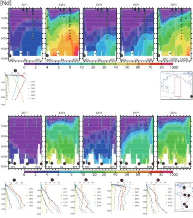
Fig. 3. VerticalεNdsections for all simulations, in the Pacific basin averaged between 120◦W and 160◦W (upper panel), and along the

western section of the Atlantic basin (lower panel). Superimposed circles are the data from the compilation by F. Lacan and T. van de Flierdt; http://www.legos.obs-mip.fr/fr/equipes/geomar/results/database may06.xls (Piepgras et Wasserburg, 1982; Piepgras et Wasserburg, 1983; Stordal et Wasserburg, 1986; Piepgras et Wasserburg, 1987; Piepgras et Jacobsen, 1989; Jeandel, 1993; Jeandel et al., 1998; Lacan et Jeandel, 2001, Amakawa et al., 2004). Colour scales are the same for all simulations and data, but different for each section. For each basin, characteristic profiles are numbered and located on the associated map, and at the bottom of each transect, for each experiment. Main characteristics for each experiment are summarized in Table 1.

this simulation succeeds in keeping a realistic isotopic sig-nature of AAIW and NADW in the Atlantic basin, although generating an AABW which is slightly too non-radiogenic (Fig. 3).

Finally in the last experiment (EXP5) in which intensity of the BE flux and values of partition coefficients of large parti-cles have been adjusted, we simulateεNddistribution in good

agreement with the data (71% fit into theεNd (model)=εNd

(data)±3εNd envelop, Figs. 3, 4, 7 and 8). In particular,

inter-basinεNd gradients (Fig. 8) and isotopic signature of

the main water masses (Fig. 3) are correctly reproduced, as well as surface isotopic signatures (Fig. 7). The increase of the Nd sink has been compensated by an increase of the sed-iment remobilization process (Fsed)to produce more

Atlantic

Pacific

Indian

ε

EXP1 EXP2 EXP3

EXP5 EXP4

data

model

data

model

data

model

data

model

data

model

0

-200

-1000

-3000

-5000 10

-20 -10 0

10

-20 -10 0

10

-20 -10 0

10

-20 -10 0

10

-20 -10 0

10

-20 -10 0

10

-20 -10 0

10

-20 -10 0

10

-20 -10 0

10

-20 -10 0

Fig. 4.εNdmodel/data cross plot for each experiment as a function of depth (colour code). Circles represent the data located in the Atlantic

basin; squares are data in the Indian basin and triangles are data in the Pacific basin. Red line is the linear interpolation line. Black lines represent the linesε_Nd(model)=ε_Nd(data) andε_Nd(model)=ε_Nd(data)±3ε_Nd, which represents a characteristic value used to define a good agreement between the model and the data. Main characteristics for each experiment are summarized in Table 1. Data are from the compilation by F. Lacan and T. van de Flierdt; http://www.legos.obs-mip.fr/fr/equipes/geomar/results/database may06.xls (see references therein).

in the [Nd] (data)±10 pmol/kg envelop). As observed in EXP4, the scavenging onto big particles leads to more coher-ent vertical gradicoher-ents, even if conccoher-entrations in the surface layer remain systematically too low (Figs. 5 and 9) while concentrations generated at high northern latitudes are too high (Figs. 5, 6 and 9). Residence time is 360 years.

5 Discussion

5.1 Sensitivity of Nd oceanic cycle to sources

The above results provide valuable information about the role (or impact) of the different Nd sources on the oceanic Nd IC and concentration distributions. This information allows a better understanding of one important aspects of the Nd paradox: how can we explain the observed Nd IC gradient along the global thermohaline circulation despite a relatively small increase in Nd concentration?

In our first experiment, we first applied dissolved river dis-charge and atmospheric dust (Fsurf – EXP1). This lead to

simulatedεNdvalues that are close to the existing data at

sur-face depths (0–200 m, Fig. 7), suggesting that these sources could control the isotopic Nd distribution in the upper ocean. However, it produces anεNddistribution that is too

homoge-neous in the deep ocean, too negative in the deep Pacific, and provides a very poor simulation of water masses signature in

the Atlantic Ocean. A possible way to improve the results in the Pacific Ocean would be to enhance vertical cycling (ei-ther by increasing the equilibrium partition coefficient for the small particles or by inserting the big particles in the scav-enging model), in order to export a radiogenic surface water-like signature at depth. However, this action yielded an in-crease in Nd sedimentation and subsequently a dein-crease in global Nd concentration. Since the simulated Nd concentra-tions in EXP1 are already an order of magnitude lower than the observed concentrations, increasing the vertical cycling does not help to reconcile both Nd IC and concentration dis-tributions, as much as the sources are restricted to the surface only.

Another option for improving the simulated deep Pa-cific and Atlantic εNd distributions was to consider an

ad-ditional source of Nd to the oceanic reservoir. Sediment re-dissolution effects along the continental margin (Boundary Source) have been tested in the second experiment (EXP2). Sediment flux (S(NdT)sed)intensity was estimated using first

1000

2000

5000 4000 3000

1000

2000

5000 4000 3000

PAC 120W - 160W

Western ATL section

3

1 2 4

5

1

1000

4000 3000 2000

5000

0 10 20 30 0 10 20 30 40

1000

4000 3000 2000

5000 Data

EXP3 EXP2

EXP4 EXP5 EXP1

Data

EXP3 EXP2

EXP4 EXP5 EXP1

0 10 20 30 40

1000

4000 3000 2000

5000

0 10 20 30

1000

4000 3000 2000 Data

EXP3 EXP2

EXP4 EXP5 EXP1

Data

EXP3 EXP2

EXP4 EXP5 EXP1

0 10 20 30 40

1000

4000 3000 2000

5000

Data

EXP3 EXP2

EXP4 EXP5 EXP1

1 2 3 4 5

1000

4000 3000 2000

0 10 120 30

1 1 1 1 1

3

1 _{2 4} 1 2 ₃ 4 1 2 3 4 1 2 3 4 1 2 3 4

Data

EXP3 EXP2

EXP4 EXP5 EXP1

EXP1 EXP2 EXP3 EXP4 EXP5

EXP1 EXP2 EXP3 EXP4 EXP5

[Nd]

4 6 8 10 20 30 40 50 60 70 80 1000

0 2

4 6 8 10 20 30 40 50 60 70 80 1000

0 2

Fig. 5. Same figure as Fig. 3, for Nd concentration (in pmol/kg).

The Nd oceanic budget simulated here suggests a large predominance (about twenty times higher than cumulated other sources) of the role of the sediment re-dissolution source (S(NdT)sed), meanwhile surface sources (S(NdT)surf)

appeared predominant for constraining surface water isotopic signatures. Other experiments, not reported here, showed that considering BE only, excluding dissolved river and dust inputs, have led to less realistic simulations of the surfaceεNd

distribution. As a source that influences Nd concentration and Nd IC at depth, we can preclude submarine groundwater as acting in the Boundary Sources, because their influence is mainly limited to the upper 200 m (Johannesson and Burdige, 2007).

Changing the solubility of atmospheric dust entering sea-water or reducing the subtraction of dissolved material in the estuaries (which would contradict the field or experimental results) may change the S(NdT)surfvalue. However, this

lat-ter value still remains small compared to S(NdT)sed value,

Atlantic

Pacific

Indian

[Nd]

EXP1 EXP2 EXP3

EXP5 EXP4

data

model

data

model

data

model

data

model

data

model

0

-200

-1000

-3000

-5000

80

0 20 40 60 80

0 20 40 60

80

0 20 40 60 80

0 20 40 60

80

0 20 40 60 80

0 20 40 60 80

0 20 40 60 80

0 20 40 60

80

0 20 40 60 80

0 20 40 60

Fig. 6. Same figure as Fig. 4, for Nd concentration (in pmol/kg). Black lines represent the lines [Nd] (model)=[Nd] (data) and [Nd]

(model)=[Nd] (data)±10 pmol/kg, which represents a characteristic value used to define a good agreement between the model and the data.

180°W 120°W 60°W 0° 60°E 120°E 180°E 60°N

0°

60°S

180°W 120°W 60°W 0° 60°E 120°E 180°E 60°N

0°

60°S

180°W 120°W 60°W 0° 60°E 120°E 180°E 60°N

0°

60°S

180°W 120°W 60°W 0° 60°E 120°E 180°E 60°N

0°

60°S

180°W 120°W 60°W 0° 60°E 120°E 180°E 60°N

0°

60°S

EXP1 EXP2

EXP3

EXP5

EXP4

0 - 200 m

ε

13

-30 -20 -15 -10 -5 0 5 2.5 -2.5 -7.5 -12.5 -17.5

Fig. 7. HorizontalεNdmaps averaged between 0 and 200 m, for all the experiments. Superimposed circles represent the data at the same

180°W 120°W 60°W 0° 60°E 120°E 180°E 60°N

0°

60°S

180°W 120°W 60°W 0° 60°E 120°E 180°E 60°N

0°

60°S

180°W 120°W 60°W 0° 60°E 120°E 180°E 60°N

0°

60°S

180°W 120°W 60°W 0° 60°E 120°E 180°E 60°N

0°

60°S

180°W 120°W 60°W 0° 60°E 120°E 180°E 60°N

0°

60°S

EXP1 EXP2

EXP3

EXP5

EXP4 2500 - 4000 m

ε

13

-30 -20 -15 -10 -5 0 5 2.5 -2.5 -7.5

-12.5 -17.5

Fig. 8. Same figure as Fig. 7, withεNdaveraged between 2500 and 4000 m.

[Nd]

(in pmol/kg)

180°W 120°W 60°W 0° 60°E 120°E 180°E 60°N

0°

60°S

180°W 120°W 60°W 0° 60°E 120°E 180°E 60°N

0°

60°S

60°N

0°

60°S

180°W 120°W 60°W 0° 60°E 120°E 180°E 60°N

0°

60°S

180°W 120°W 60°W 0° 60°E 120°E 180°E 60°N

0°

60°S

EXP1 EXP2

EXP3

EXP5

EXP4 0 - 200 m

60

0 2 6 10 14 18 40 20 16 12 8 4

Fig. 9. Same figure as Fig. 7, for Nd concentration (in pmol/kg).

5.2 Sensitivity of Nd oceanic cycle to vertical cycling:

small vs. big particles

The second experiment successfully simulated reasonable distributions of both Nd IC and concentrations. However, some discrepancies still remain, particularly in the deep Pa-cific where simulated deep waters had underestimated Nd IC and overestimated concentrations. Enhancing vertical

cy-cling in order to homogenize the vertical column in the Pa-cific is therefore pertinent, though it should maintain the out-come in the Atlantic Ocean. As the lateral isopycnal trans-port is more intense in the Atlantic than in the Pacific Ocean, vertical processes in this last basin might be more sensitive.

[Nd]

(in pmol/kg)

180°W 120°W 60°W 0° 60°E 120°E 180°E 60°N

0°

60°S

180°W 120°W 60°W 0° 60°E 120°E 180°E 60°N

0°

60°S

180°W 120°W 60°W 0° 60°E 120°E 180°E 60°N

0°

60°S

180°W 120°W 60°W 0° 60°E 120°E 180°E 60°N

0°

60°S

180°W 120°W 60°W 0° 60°E 120°E 180°E 60°N

0°

60°S

EXP1 EXP2

EXP4 2500 - 4000 m

60

0 2 6 10 14 18 40 20 16 12 8 4

Fig. 10. Same figure as Fig. 8, for Nd concentration (in pmol/kg).

100°W 0° 100°E 80°N

40°N

0°

40°S

-2.5

-7 -6 -5 -4 -3 -3.5

-4.5

-5.5

-6.5

Fig. 11. Logarithmic map of Nd flux to the seafloor for experience

EXP5, in g m−2yr−1. Black line delineates the continental margin area, where 64% of the Nd sink is located.

cycling, either by increasing the partition coefficient for small particles (EXP3) or by inserting big particles in the reversible scavenging model (EXP4), increases the removal of Nd from the water column and reduces our global Nd con-centration to more unrealistic values (cf. Table 1, Figs. 5, 6, 9 and 10).

Both EXP3 and EXP4 successfully generated the required reduction of Nd concentration, and the formation of more ra-diogenic waters in the deep Pacific Ocean (Figs. 3, 4 and 8). However they differed in their performance in the Atlantic Ocean. EXP3 generated a significant degradation of simu-latedεNdcharacteristics in the Atlantic Ocean, while EXP4

preserved and even improved agreement with the data in the Atlantic basin.

These results are consistent with those of Siddall et al. (2008), which demonstrated the importance of vertical cycling (reversible scavenging process) in reconciling Nd IC and concentration distributions, and therefore resolving the “Nd paradox”. Also, this highlights the importance of differ-ent pools of particles size in this model for setting the char-acteristics of the Nd isotopic distribution, and more precisely the potential role of fast sinking particles.

5.3 The “Nd paradox”

Based on information gained from previous sensitivity tests on sources and vertical cycling (EXP1 to EXP4), the configuration of our last experiment (EXP5) was adjusted to obtain the best agreement between simu-lations and data. We have considered the surface sources of EXP1 (S(NdT)surf=2.6×108g(Nd)/yr) whereas

the sediment remobilization has been slightly increased (S(NdT)sed=1.1×1010g(Nd)/yr), in order to compensate for

the decrease in Nd concentration caused by the insertion of big particles in the reversible scavenging model. Associated with this later source, the sink of Nd along the continental margin (corresponding to the Boundary Scavenging process), even if less important as the source, represents as much as 64% of the global Nd sink (Fig. 11), confirming that BE acts as both a major source and sink for oceanic Nd, as deduced from the observations (Lacan and Jeandel, 2005).

not necessarily optimal, but it shows some improvements compared to the four other experiments. The resulting simu-lated Nd IC is in excellent agreement with the observed data (Figs. 3, 4, 7 and 8), though concentrations in the surface ocean are low (Figs. 5, 6 and 9). We attribute this bias to the particulate fields generated by the biogeochemical model PISCES. In this work, as in the 231Pa and 230Th simula-tions proposed by Dutay et al. (2009), and consistent with either experimental or field observations, the small particle pool drives the vertical cycling in the water column. It is characterized here with a higher equilibrium coefficient for small particles than for the big particle pool. However, small particle fields generated by PISCES are underestimated at depth (Dutay et al., 2009) leading to an overestimation of the Nd concentrations (as Nd is less scavenged). Improv-ing the small particle concentration at depth in the PISCES model would likely help to smooth the vertical modelled gra-dient, recover deep Pacific radiogenic waters in our simula-tion (Figs. 3 and 8), and better simulate element cycles in the ocean, which is an important goal. Nevertheless, in our model, big particles also play an important role in reconcil-ing deep ocean Nd concentration while keepreconcil-ing the Nd IC as a water-mass tracer property.

The residence time of Nd in the ocean in this last experi-ment is 360 years, which is in the lower range of previous es-timations of∼300 to∼600 years (Piepgras and Wasserburg, 1983; Jeandel et al., 1995; Tachikawa et al., 1999, 2003; Sid-dall et al., 2008). This value is still consistent with the con-servativity ofεNdwithin the major oceanic water masses. All

together, these factors suggest that i) the Boundary Source is a major primordial source for Nd oceanic cycle (∼95% of the global sources), ii) Boundary Scavenging, resulting from vertical cycling in margin areas, is a major sink (64% of the global sink), and iii) vertical cycling in the open ocean is es-sential for the redistribution of Nd and its IC within the ocean interior. While the two first points provide an explanation for the BE observed in field data, the three points provide a means to reconcile the “Nd paradox”. The first estimation of the order of magnitude of the “missing flux” proposed by Tachikawa et al. (2003) is confirmed by our model results. The reversible scavenging is also essential to explain the Nd nutrient-like profile in the water column and the water mass tracer property of Nd IC, in agreement with recent REE mod-elling studies (Nozali and Alibo, 2003; Siddall et al., 2008; Oka et al., 2008).

However, if Boundary Sources are found to explain the large Nd IC variation observed along the global thermohaline circulation, without a large Nd concentration change (due to the associated Boundary Scavenging, Fig. 11), the question of why there is an apparent contradiction between conserva-tive Nd IC and non conservaconserva-tive Nd concentrations remains to be solved. This critical point should be addressed in an-other dedicated study, so as to fully resolve the “Nd para-dox”.

6 Conclusions

The objective of this study was to use an ocean model as a tool to better understand the Nd oceanic cycle and to work toward the resolution of the “Nd paradox”, (i.e. estimating the sources and sink of the element, and qualifying the pro-cesses acting on the element’s distribution within the reser-voir). We simultaneously simulated both Nd isotopic compo-sition and concentration using a prognostic coupled dynam-ical/biogeochemical model and used a reversible scavenging model to simulate the Nd transformation and sink into the ocean. We have also implemented for the first time a realis-tic calculation of the Nd sources, with an explicit representa-tion of sedimentary remobilizarepresenta-tion along continental margins (source of the Boundary Exchange process) as well as dis-solved river discharge and atmospheric dust sources (surface sources).

In accordance with previous results of Siddall et al. (2008) and Oka et al. (2008), vertical cycling needs to be invoked (surface removal combined with remineralisation at depth) to correctly simulate Nd isotopic composition and concen-tration distributions. As yet, we are unable to verify the va-lidity of our partition coefficients because very little data are available. A strong recommendation deduced from this work is to improve our knowledge of the dissolved/particle distri-bution of the geochemical tracers, which the GEOTRACES program should make possible. Our performance in simulat-ing Nd concentration is also still limited by our models. In particular, the low concentration in the small particles field simulated at depth by the PISCES model is very likely the cause for overestimated Nd concentration surface to depth gradients. This work also suggests that regarding the pa-rameterization used and the particle distribution generated by the biogeochemical model, it is important to consider differ-ent kinds of particles, and especially their sinking velocity, in setting the characteristics of the Nd isotopic distribution. This study can therefore be used as a basis for improving the representation of the complexity of observed particle field distribution in the model, such as considering a whole con-tinuous spectrum of particle size (Gehlen et al., 2006).

dissolution (3–5%) required to obtain these fluxes. Dissolved river discharge (2.6×108g(Nd)/yr), and atmospheric dusts (1.0×108g(Nd)/yr) play a significant role only on surface

εNddistribution. The residence time of Nd in the ocean,

cal-culated in this configuration, is estimated to be 360 years, which is in agreement with previous estimates.

The high computational cost for one simulation was a lim-iting factor for sensitivity tests on sources and equilibrium partition coefficients. Optimal values of parameters of the model may not be those used for experiment EXP5, but we are confident that our main results are robust. One easily en-visaged improvement could be the use of the Transport Ma-trix Method (Khatiwala et al., 2005) for this model, to better optimize these parameters.

This study highlights the predominant role of Boundary Exchange on Nd oceanic cycle, and suggests Nd isotopes as a powerful tool to quantify margin source to the ocean, which may have significance for the general ocean chemistry. However, we have no indication of chemical, biological or physical processes that act on this sediment re-dissolution. Particularly, one of the main shortcomings resides in the as-sumption that the input from the margin is set geographi-cally constant, whereas some factors can act on the source (oxygen concentration, currents velocity, turbulence, temper-ature, organic matter deposition, etc...), leading to potentially large variations. It then appears to be quite important for the geochemical community to pay attention at continental margins/open ocean interfaces to determine if the “Boundary Scavenging” (observed for Be and Pa/Th, Anderson et al., 1990) is compensated by lithogenic inputs for other chemi-cal tracers, and how this input is materialized (e.g. cold hy-drothermalism on margins, remobilization and dissolution of sediments after resuspension, early diagenesis or both, water penetration in sediments, etc. . . ).

This implies the need for a multi-tracer approach, in par-ticular with highly reactive elements such as231Pa and230Th. Also, it seems inevitable to improve and adapt biogeochem-ical models to the simulation of trace elements, including iron manganese hydroxides and oxide crusts that are hypoth-esized to be main carriers of these tracers.

Acknowledgements. We thank B. O’Shea and K. Jones for the

linguistic advice. We also thank F. Joos, M. Siddall and two anonymous reviewer for their careful reading of the manuscript and helpful remarks.

Edited by: F. Joos

The publication of this article is financed by CNRS-INSU.

References

Amakawa, H., Nozaki, Y., Alibo, D. S., Zhang, J., Fukugawa, K., and Nagai, H.: Neodymium isotopic variations in Northwest Pa-cific waters, Geochim. Cosmochim. Ac., 68, 715–727, 2004. Anderson, R. F., Lao, Y., Broecker, W. S., Trumbore, S. E.,

Hof-mann, H. J., and Wolfli, W.: Boundary scavenging in the Pacific Ocean: a comparison of10Be and231Pa, Earth Planet. Sci. Lett., 96, 287–304, 1990.

Arsouze, T., Dutay, J. C., Lacan, F., and Jeandel, C.: Modeling the neodymium isotopic composition with a global ocean circulation model, Chem. Geol., 239, 165–177, 2007.

Arsouze, T., Dutay, J.-C., Kageyama, M., Lacan, F., Alkama, R., Marti, O., and Jeandel, C.: A modeling sensitivity study of the influence of the Atlantic meridional overturning circulation on neodymium isotopic composition at the Last Glacial Maximum, Clim. Past, 4, 191–203, 2008,

http://www.clim-past.net/4/191/2008/.

Aumont, O., Maier-Reimer, E., Blain, S., and Monfray, P.: An ecosystem model of the global ocean including Fe, Si, P colimitations, Global Biogeochem. Cy., 17(2), 1060, doi:10.1029/2001GB001745, 2003.

Aumont, O. and Bopp, L.: Globalizing results from ocean in situ iron fertilization studies, Global Biogeochem. Cy., 20, GB2017, doi:10.1029/2005GB002591, 2006.

Bacon, M. P. and Anderson, R. F.: Distribution of thorium iso-topes between dissolved and particulate forms in the Deep-Sea., J. Geophys. Res., 87, 2045–2056, 1982.

Bayon, G., German, C. R., Burton, K. W., Nesbitt, R. W., and Rogers, N.: Sedimentary Fe-Mn oxyhydroxides as paleoceano-graphic archives and the role of aeolian flux in regulating oceanic dissolved REE, Earth Planet. Sci. Lett., 224, 477–492, 2004. Bertram, C. J. and Elderfield, H.: The geochemical balance of the

rare earth elements and Nd isotopes in the oceans, Geochim. Cos-mochim. Ac., 57, 1957–1986, 1993.

Blanke, B. and Delecluse, P.: Variability Of The Tropical Atlantic-Ocean Simulated By A General-Circulation Model With 2 Dif-ferent Mixed-Layer Physics, J. Phys. Oceanogr., 23, 1363–1388, 1993.

Boillot, G. and Coulon, C.: La d´echirure continentale et l’ouverture oc´eanique - G´eologie des marges passives, Overseas Publish-ers Association eds., Gordon and Breach Science PublishPublish-ers ed., 1998.

Broecker, W. S. and Peng, T. H.: Tracers in the Sea, Eldigio Press, Palisades, NY, 690 pp., 1982.

Dahlqvist, R., Andersson, P. S., and Ingri, J.: The concentration and isotopic composition of diffusible Nd in fresh and marine waters, Earth Planet. Sci. Lett., 233, 9–16, 2005.

Doney, S. C., Lindsay, K., Caldeira, K., Campin, J. M., Drange, H., Dutay, J. C., Follows, M., Gao, Y., Gnanadesikan, A., Gru-ber, N., Ishida, A., Joos, F., Madec, G., Maier-Reimer, E., Marshall, J. C., Matear, R. J., Monfray, P., Mouchet, A., Naj-jar, R., Orr, J. C., Plattner, G. K., Sarmiento, J., Schlitzer, R., Slater, R., Totterdell, I. J., Weirig, M. F., Yamanaka, Y., and Yool, A.: Evaluating global ocean carbon models: The impor-tance of realistic physics, Global Biogeochem. Cy., 18, GB3017, doi:10.1029/2003GB002150, 2004.

T. D., Knap, A. H., Reinhardt, K. H., Schneider, B., Soudine, A., Tokos, J. J., Tsunogai, S., Wollast, R., and Zhou, M.: The atmospheric input of trace species to the world ocean, Global Biogeochem. Cy., 5, 193–259, 1991.

Dutay, J. C., Bullister, J. L., Doney, S. C., Orr, J. C., Najjar, R., Caldeira, K., Campin, J. M., Drange, H., Follows, M., Gao, Y., Gruberi, N., Hecht, M. W., Ishida, A., Joos, F., Lindsay, K., Madec, G., Maier-Reimer, E., Marshall, J. C., Matear, R. J., Monfray, P., Mouchet, A., Plattner, G.-K., Sarmiento, J., Schlitzer, R., Slater, R., Totterdell, I. J., Weirig, M.-F., Ya-manaka, Y., and Yool, A.: Evaluation of ocean model ventila-tion with CFC-11: comparison of 13 global ocean models, Ocean Model., 42, 89–120, 2002.

Dutay, J. C., Jean-Baptiste, P., Campin, J. M., Ishida, A., Maier-Reimer, E., Matear, R. J., Mouchet, A., Totterdell, I. J., Ya-manaka, Y., Rodgers, K., Madec, G., and Orr, J. C.: Evaluation of OCMIP-2 ocean models’ deep circulation with mantle helium-3, J. Marine Syst., 48, 15–36, 2004.

Dutay, J.-C., Lacan, F., Roy-Barman, M., and Bopp, L.: Influ-ence of particle size and type on 231 Pa and 230 Th simulation with a global coupled biogeochemical-ocean general circulation model: A first approach, Geochem. Geophy. Geosy., 10, Q01011, doi:10.1029/2008GC002291, 2009.

Elderfield, H.: The oceanic chemistry of the Rare Earth Elements, Philos. T. Roy. Soc. Lond., 325, 105–106, 1988.

Elderfield, H., Upstill-Goddard, R., and Sholkovitz, E. R.: The rare earth elements in rivers, estuaries, and coastal seas and their significance to the composition of ocean waters, Geochim. Cos-mochim. Ac., 54, 971–991, 1990.

Fichefet, T. and Maqueda, M. A. M.: Sensitivity of a global sea ice model to the treatment of ice thermodynamics and dynamics, J. Geophys. Res.-Oceans, 102, 12609–12646, 1997.

Gehlen, M., Bopp, L., Emprin, N., Aumont, O., Heinze, C., and Ragueneau, O.: Reconciling surface ocean productivity, export fluxes and sediment composition in a global biogeochemical ocean model, Biogeosciences, 3, 521–537, 2006,

http://www.biogeosciences.net/3/521/2006/.

Gent, P. R. and McWilliams, J. C.: Isopycnal Mixing In Ocean Cir-culation Models, J. Phys. Oceanogr., 20, 150–155, 1990. GEOTRACES: An international study of the marine

biogeochem-ical cycles of trace elements and isotopes, online available at: http://www.geotraces.org/, 2005.

Goldstein, S. L., O’Nions, R. K., and Hamilton, P. J.: A Sm-Nd study of atmospheric dusts and particulates from major river sys-tems, Earth Planet. Sci. Lett., 70, 221–236, 1984.

Goldstein, S. L. and Jacobsen, S. B.: The Nd and Sr isotopic sys-tematics of river-water dissolved material: implications for the sources of Nd and Sr in the seawater, Chem. Geol. (Isotope Geosc. Section), 66, 245–272, 1987.

Goldstein, S. L. and Hemming, S. R.: Long lived Isotopic Trac-ers in Oceanography, Paleoceanography, and Ice sheet dynamics, in: Treatise on Geochemistry, edited by: Elderfield, H., Elsevier Pergamon press, Amsterdam, chapter 6.17, 2003.

Greaves, M. J., Statham, P. J., and Elderfield, H.: Rare earth element mobilization from marine atmospheric dust into seawater, Mar. Chem., 46, 255–260, 1994.

Grousset, F., Parra, M., Bory, A., Martinez, P., Bertrand, P., Shiem-mield, G., and Ellam, R. M.: Saharan wind regimes traced by the Sr-Nd isotopic composition of subtropical Atlantic Sediments:

last glacial maximum vs. today, Quaternary Sci. Rev., 17, 395– 409, 1998.

Grousset, F. E., Biscaye, P. E., Zindler, A., Prospero, J., and Chester, R.: Neodymium isotopes as tracers in marine sediments and aerosols: North Atlantic, Earth Planet. Sci. Lett., 87, 367–378, 1988.

Gutjahr, M., Frank, M., Stirling, C. H., Keigwin, L. D., and Hall-iday, A. N.: Tracing the Nd isotope evolution of North Atlantic deep and intermediate waters in the Western North Atlantic since the Last Glacial Maximum from Blake Ridge sediments, Earth Planet. Sci. Lett., 266, 61–77, 2008.

Henderson, G. M., Heinze, C., Anderson, R. F., and Winguth, A. M. E.: Global distribution of the Th-230 flux to ocean sediments constrained by GCM modelling, Deep-Sea Res. I, 46, 1861– 1893, 1999.

Jeandel, C.: Concentration and isotopic composition of Nd in the South Atlantic Ocean, Earth Planet. Sci. Lett., 117, 581–591, 1993.

Jeandel, C., Bishop, J. K., and Zindler, A.: Exchange of Nd and its isotopes between seawater small and large particles in the Sar-gasso Sea, Geochim. Cosmochim. Ac., 59, 535–547, 1995. Jeandel, C., Thouron, D., and Fieux, M.: Concentrations and

Iso-topic compositions of Nd in the Eastern Indian Ocean and In-donesian Straits, Geochim. Cosmochim. Ac., 62, 2597–2607, 1998.

Jeandel, C., Arsouze, T., Lacan, F., Techine, P., and Dutay, J. C.: Isotopic Nd compositions and concentrations of the lithogenic inputs into the ocean: A compilation, with an emphasis on the margins, Chem. Geol., 239, 156–164, 2007.

Johannesson, K. H. and Burdige, D. J.: Balancing the global oceanic neodymium budget: Evaluating the role of groundwater, Earth Planet. Sci. Lett., 253, 129–142, 2007.

Jones, K., Khatiwala, S., Goldstein, S. L., Hemming, S. R., and Van de Flierdt, T.: Modeling the distribution of Nd isotopes in the oceans using an offline Ocean General Circulation Model, Earth Planet. Sci. Lett., 202(3–4), 610–619, 2008.

Khatiwala, S., Visbeck, M., and Cane, M. A.: Accelerated sim-ulation of passive tracers in ocean circsim-ulation models, Ocean Model., 9, 51–69, 2005.

Kriest, I.: Different parameterizations of marine snow in a 1D-model and their influence on representation of marine snow, ni-trogen budget and sedimentation, Deep-Sea Res. I, 49, 2133– 2162, 2002.

Lacan, F. and Jeandel, C.: Tracing Papua New Guinea imprint on the central Equatorial Pacific Ocean using neodymium isotopic compositions and Rare Earth Element patterns, Earth Planet. Sci. Lett., 186, 497–512, 2001.

Lacan, F. and Jeandel, C.: Subpolar Mode Water formation traced by neodymium isotopic composition, Geophys. Res. Lett., 31, L14306, doi:10.1029/2004GL019747, 2004.

Lacan, F. and Jeandel, C.: Neodymium isotopes as a new tool for quantifying exchange fluxes at the continent – ocean interface, Earth Planet. Sci. Lett., 232, 245–257, 2005.

Madec, G.: NEMO reference manual, ocean dynamics component : NEMO-OPA. Preliminary version, Note du Pole de mod´elisation, Institut Pierre-Simon Laplace (IPSL), 27, 2006.

Monod, J.: Recherches sur la croissance des cultures bact´eriennes, Hermann, Paris, 1942.