Electron temperature in nighttime sporadic E layer at mid-latitude

Ann. Geophys., 26, 533–541, 2008 www.ann-geophys.net/26/533/2008/ © European Geosciences Union 2008

Annales

Geophysicae

Electron temperature in nighttime sporadic E layer at mid-latitude

K.-I. Oyama1, T. Abe2, H. Mori3, and J. Y. Liu1

1_{Institute of Space Science, National Central University, Jhongda Rd., Jhongli, Taiwan}

2_{Institute of Space and Astronautical Science/Japan Space Exploration Agency, 3-1-1, Yoshinodai, Sagamihara, Japan} 3_{National Institute of Information and Communications Technology, 4-2-1, Nukui-kitamachi, Koganei, Tokyo, Japan}

Received: 31 July 2007 – Revised: 17 December 2007 – Accepted: 17 January 2008 – Published: 26 March 2008

Abstract. Electron temperature in the sporadic E layer was measured with a glass-sealed Langmuir probe at a mid-latitude station in Japan in the framework of the SEEK (Spo-radic E Experiment over Kyushu)-2 campaign which was conducted in August 2002. Important findings are two fold: (1) electron temperature and electron density vary in the op-posite sense in the height range of 100–108 km, and elec-tron temperature in theEs layer is lower than that of ambi-ent plasma, (2) electron temperature in these height ranges is higher than the possible range of neutral temperature.

These findings strongly suggest that the heat source that elevates electron temperature much higher than possible neu-tral temperature exists at around 100 km, and/or that the physical parameter values, which are used in the present the-ory to calculate electron temperature, are not proper. Keywords. Ionosphere (Ionospheric irregularities; Mid-latitude ionosphere)

1 Introduction

To measure electron temperature (Te)inside sporadicE(Es) is a difficult task because sounding rockets go through thin layer(s) where electron density changes very fast. To obtain

Te in the nighttimeEs, together with that outsideEs from Langmuir probe, is especially difficult or almost impossible when the electron density (Ne)is not high enough and the amplifier of the instrument does not have enough gain with the sufficient frequency response. In addition, the v-i charac-teristic curve of the Langmuir probe is distorted by the spin-ning of the rocket and/or by the irregular electron density structure if the probe sweep bias is not fast enough. To ob-tain an accurate v-i characteristic curve in the rapidly chang-ing media, a well-designed instrument is needed, as well as careful laboratory experiments.

Correspondence to: K.-I. Oyama

([email protected])

For these reasons, only fewTe data exist so far. Schutz and Smith (1976) reported Te of 520 K inside the Es lay-ers at the heights of 108.5 km and 114.5 km. Teoutside was 550 K at 106.5 km and 111.5 km, which means that Te in-sideEs was about 30 K lower than the ambient plasma. This result was obtained by simply averaging 29 points ofTe val-ues, which were measured in the height range of 105 km– 125 km. No detailed analysis of the rocket attitude was con-ducted. Szuszczewicz and Holmes (1977) reportedTeinside Es in the height range of 105–107 km, both for up leg and down leg. In the up leg,Nestarts increasing at the height of 106.0 km, and takes a peak at the height of 106.71 km, and then decreases. Te at the peakNe was 345 K, andTe at the height of 107.5 km was 380 K. For the down leg, the height of

Nemaximum was 106.2 km. Below theNemaximum that is found at the height of 105.7 km,Tewas 345 K and above the maximumNeat the height of 106.5 km,Tewas 500 K. Thus, TeinsideEs is 140 K lower than outsideEs. Two other pa-pers reported onTe insideEs. Aubry et al. (1966) showed twoEs events. One case is thatTe insideEs was 1/2 that of the ambient. Another case is thatTeis two times higher than the ambient. Andreyeva et al. (1971) reported two cases; one case showsTeinsideEs equal to that of outsideEs, and the other case indicatesTe insideEs is 10% lower than that of the ambient.

Gleeson and Axford (1967) conducted theoretical discus-sion by taking the heating due to the internal gravity wave into account.Tein the midst ofEs, which was located at the height of 115 km, was calculated to be about 90 K lower than that of the ambient.

534 K.-I. Oyama et al.: Electron temperature in nighttime sporadic E layer at mid-latitude

12

Fig 1. Cartoon of the glas sealed Langmuir electrode

Fig 1. Cartoon of Glass sealed Langmuir Probe

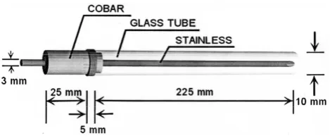
“Support rod” which is mentioned in Fig2a is made of COVAR (iron-nickel alloy, 25mm in length, and 10mm outer diameter).

Fig. 1. Diagram of glass-sealed Langmuir probe sensor “support

rod”, which is mentioned in Fig. 2a, and made of COVAR (25 mm in length, and 10 mm outer diameter).

2 Instrumentation

Special attention should be paid to be electrode and the elec-tronics, in order to obtain an accurate value from the Lang-muir probe measurement, although the principle itself of the measurement is very simple. The contamination of the electrode surface is most serious problem (Oyama, 1976). To avoid the effect of the electrode contamination, a glass-sealed Langmuir probe ,which consists of a cylindrical stain-less electrode and a glass tube, was used (Oyama and Hirao, 1976). A cylindrical stainlesssteel electrode of 3 mm in di-ameter and 22.5 cm long was installed in the glass tube with an inner diameter of 9 mm and outer diameter of 10 mm (see Fig. 1). The glass tube was connected to the turbo-molecular pump, and the tube was evacuated inside. During the evac-uation, under the pressure of less than 1×10−7_{Torr, the} sys-tem, including electrode and the glass tube, was baked. It is essential to heat the electrode higher than 100◦_{C, because the} main contaminant is water. It is highly recommended that the temperature of the electrode and glass tube should be 160– 200◦C. After the evacuation, 2–3 days later, the end of the glass tube was cut from the vacuum system and the cylinder electrode was sealed in the glass tube. Without these proce-dures, it is impossible to remove the electrode contaminants, which usually cover the surface of the electrode.

Probe voltage in a triangular shape was swept from 0 V to 2.5 V and then from 2.5 V to 0 V within 0.25 s, which pro-vided one v-i characteristic curve every 0.125 s. The use of the triangular wave allows us to check the hysteresis of the v-i curve (Oyama, 1976). The hysteresis appears when the electrode is contaminated. The small hysteresis of the v-i curve is also produced in the measurement system itself. It originates from the stray capacitance of the cable, connecting the electronics and the electrode. The amplifier itself causes the second hysteresis, if the frequency response is limited to a low frequency. The hysteresis should be eliminated, in order to obtain an accurateTe. To remove the hysteresis associated with the stray capacitance, the sweep voltage is applied to the outer shielding cable. This finally leads to no accumula-tion of the electronic charge between the center wire and the outer shielding cable. In order to remove the amplifier

hys-teresis, the amplifier needs enough of a frequency response. One should note that it is impossible to obtain an accurate electron temperature without special attention regarding the electrode and the electronics.

3 Rocket experiment

The S-310-31 rocket was launched at 23:24 JST on 3 Au-gust 2002, to study the QP echo associated with sporadic E from the Kagoshima Space Center (131◦050E, 31◦150N in geographic coordination). The second rocket, S-310-32, was launched 15 min after the first rocket. Adjusted solar radio flux and theKpindex (sum) were 172.7 and 22, respectively. A glass-sealed Langmuir probe, which was described above, was installed in the rocket S-310-31. The location of the glass-sealed Langmuir probe is illustrated in Fig. 2. The nose cone was opened 60 s after the launch at the height of 70 km. Two seconds after opening the nose cone, the root of the glass tube was destroyed by a guillotine actuated by the first squib (shown in Fig. 2 as wire cut 1); one second after the destruction of the glass tube, the second squib (shown in Fig. 2 as wire cut 2) was activated to cut the wire, which fas-tened the glass tube along the rocket spin axis, and the Lang-muir electrode was ejected perpendicularly to the rocket spin. Simultaneously, the glass tube was removed by a centrifugal force of the rocket spin.

The spin rate of the rocket was reduced from an initial spin rate of 2.2 Hz to 0.7 Hz by a yo-yo despinner 55 s after the launch at the height of 55 s. Accordingly, one v-i charac-teristic curve was obtained during about 30 degrees of rocket spin. A current amplifier picked up the probe current and the voltage-converted current was amplified with three am-plifiers. Output voltage of 5 V corresponds to 1 microampere for a low gain amplifier, 0.1 microamperes for a middle gain amplifier, and 0.01 microamperes for a high gain amplifier, respectively. The output voltages of the three amplifiers have an offset voltage of 0.5 V, in order to measure the ion current, which means that zero current corresponds to 0.5 V. A circuit was calibrated every 30 s by connecting 40 mega ohm resis-tance to the input of the amplifier right after disconnecting the wire to the electrode. An 8-bit A/D converter converted the output voltage with the sampling frequency of 3200 Hz. During 78–108 s (height: 90–120 km) after the launch, the output voltage from the middle gain amplifier was converted by 12 bits, with a sampling frequency of 6400 Hz and stored in the memory. The data, which is thus stored in the memory, was transmitted to the ground 193 s after the launch when the rocket reached approx. the apogee. The retrieval of the data was completed at 313 s after the launch.

K.-I. Oyama et al.: Electron temperature in nighttime sporadic E layer at mid-latitude 535

13

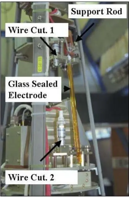
Fig.2 (a) Location of Glass sealed Langmuir Probe (indicated as Glass Sealed Electrode in the figure), and two wire cutters. Glass tube of glass sealed Langmuir probe is covered with adhesive tape so that pieces of the glass cylinder do not scatter when the glass tube is broken by the first squib (indicated as Wire Cut. 1 in the figure) at the end of the support rod, which is shown in Fig.1. The second squib (indicated as Wire Cut.2 in the figure) releases the wire, which holds the glass sealed Langmuir probe along the rocket axis.

Fig. 2a. Location of glass-sealed Langmuir Probe (indicated as

glass-sealed electrode in the figure), and two wire cutters. Glass tube of glass-sealed Langmuir probe is covered with adhesive tape, so that the pieces of the glass cylinder do not scatter when the glass tube is broken by the first squib (indicated as a wire cut 1 in the figure) at the end of the support rod, which is shown in Fig. 1. The second squib (indicated as wire cut 2 in the figure) releases the wire, which holds the glass-sealed Langmuir probe along the rocket axis.

ion current from the curve.Newas calculated in 3 ways. One is calculated by taking the electron current,i, at the inflex-ion point of the semi-log plotted i-v curve by the following equation, although argument exists on the inflection point to be defined as space potential:

Ne=i/{S·e·(kTe/2π·Me)1/2},

whereSis surface area of the cylindrical electrode,eis the electron charge, Me is the mass of electron, and k is the Boltzmann constant. Another value of electron density is obtained by normalizing the ion current atfoEs of the iono-gram observed at the nearest ionosonde station located at Ya-magawa. One more electron density was measured with a spherical Langmuir probe of a fixed bias, which gives bet-ter high resolution than the other two methods. The value is normalized by ionosonde data. Among the threeNe val-ues, the last one has the smallest spin modulation because

14

(b) Deployed Glass sealed Langmuir probe, which is perpendicular to the rocket spin axis near the top of the payload section. A fixed biased spherical electrode to measure height profiles of relative electron density and an Impedance probe to measure absolute electron density are also shown.

Fig. 2b. Deployed glass-sealed Langmuir probe, which is

perpen-dicular to the rocket spin axis near the top of the payload section. A fixed biased spherical electrode to measure the height profiles of the relative electron density and an impedance probe to measure the absolute electron density are also shown.

the sensor was located at the center of the payload top. The value from the cylindrical probe, which was deployed radial to the spin axis, is influenced strongly by the angle between the electrode and the direction of the geomagnetic field. The data were processed with respect to the spin phase and the moving direction of the rocket.

536 K.-I. Oyama et al.: Electron temperature in nighttime sporadic E layer at mid-latitude

15 (a)

(b)

(c)

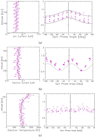
Fig.3 (a) Variation of ion current in the height range of 138.3-143.9km, (b) variation of electron current in the height range of 134.2-140.7km and (c) variation of electron temperature in the height range of 110.5-120.9 km, versus height (left), and spin phase (right). Ion and electron currents, and electron temperature are normalized by the value measured when the sensor locates at the rocket moving direction.

Fig. 3. (a) Variation of ion current in the height range of 138.3–143.9 km, (b) variation of electron current in the height range of 134.2–

140.7 km and (c) variation of electron temperature in the height range of 110.5–120.9 km, versus height (left), and spin phase (right). Ion and electron current, and electron temperature are normalized.

more pronounced near the space potential, and therefore, the effect of the geomagnetic field does not reach the floating po-tential region. Figure 3c shows that the ambiguity of theTe measurement is roughly less than 100 K.

4 Data obtained and discussion

K.-I. Oyama et al.: Electron temperature in nighttime sporadic E layer at mid-latitude 537

16

Low Gain

Ascent

Middle Gain

High Gain High Gain

Low Gain

Middle Gain

Maximum Ion Current [ǴA] Maximum Ion Current [ǴA]

Descent

Altitude [km] Altitude [km]

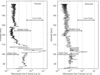
Ｆig.4 Height profile of the ion current from the v- i characteristic curve for up leg (left) and down leg (right) of the rocket trajectory. Three amplifiers of different gains measured the height profile of the ion currents. Dashed lines with arrows indicate the range of the current to be measured with three amplifiers of Low, Middle, and High gain. The rocket spinning causes fine scale fluctuation of the current. Large structure, which appears in the 100-112 km and 127-130km during upleg, shows the real structure of the ionosphere, although down leg profile is highly modulated by rocket spin, small reduction of the current, which exists at the height of 118-125 km and peak of ion current at the height of 100-107 km, are believed to be real.

Fig. 4. Height profile of the ion current from the v-i characteristic curve for the up leg (left) and the down leg (right) of the rocket trajectory.

Three amplifiers of different gains (low, middle, and high) provide the height profile of the ion current. The rocket spinning causes fine scale fluctuation in the current. The large structure, which appears in the 100–112 km and 127–130 km during up leg, shows the real structure of the ionosphere, although down leg profile is highly modulated by rocket spin, a small reduction in the current, which exists at the height of 118–122 km and the peak of the ion current at the height of 100–106 km, seems to be real.

of the sweep voltage is well in the ion saturation regime of the v-i characteristic curves.

In the height region between 100–110 km, the Es layer was found. The first maximum of 1.5×10−1µA was lo-cated at the height of 103.5 km. At the height of 105.5 km the second maximum of 9×10−2µA was found. Finally, at the height of 107 km, a thin layer of 8×10−8µA was found. After the rocket went through the Es layer between 100– 110 km, the ion current gradually reduced, reaching its min-imum at 123 km and again gradually turned to increase. At the height of 128 km the current dropped from 4×10−4µA to 1.8×10−4µA and suddenly jumped to 10−3µA at the height of 129 km and then dropped to 4×10−4µA. This peculiar behavior might be the key observation to study the forma-tion mechanism of theEs layer, as we will discuss in a sep-arate paper. A small peak is seen at the height of 142 km. This small peak can be seen more clearly in the electron cur-rent (which is not shown here) of the v-i characteristic curve. Similar structures, which exist at the heights of 100, 110, 123 and 142 km during the up leg, are also recognized at 98–108, 120 and 141 km during the down leg.

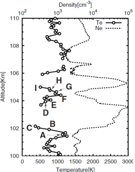
In Fig. 5, the height range of 100–110 km is expanded, whereTeis plotted together withNe.Tewas calculated from the semi-log plot of the electron current, that is measured with a cylindrical Langmuir probe. The accuracy ofTe, as

a worst case, might be about 50–100 K, taking into account all possible factors, such as spin effects, the ambiguity of curve fitting, and the frequency response of the instrument. Although the results, which have been reported earlier, also mentioned the same accuracy, the quality of our data is in-comparably excellent.

The electron current, which was measured with a fixed bi-ased spherical Langmuir probe, at the probe voltage of 4.5 V, was normalized by the upper hybrid resonance of the gyro-plasma probe (Oya, 1969) at the maximum density height of 103.5 km. The impedance probe gives reliable absolute val-ues forNehigher than 103els/cc. One can see that even small variations inTe are well anti-correlated withNe, in spite of the fact that two parameters are measured by different elec-trodes and calculated independently.

The first and second peaks ofNeat the heights of 103.5 km and 105.3 km are 105els/cc and 9×104els/cc, respectively. Just below the first peak,Neis 4×103els/cc at the height of 101.5 km. Ne between the two density peaks, at the height of 104.5 km, is 3×103els/cc. Teis 1000 K and 300 K at the heights of 101.5 km and 102 km, respectively. Above the first

Nepeak,Teis 500 K. Between the first and secondNepeaks, Teis 1000 K.

538 K.-I. Oyama et al.: Electron temperature in nighttime sporadic E layer at mid-latitude

17

Fig.5 Te (solid line with white circles) and Ne (dashed line) in the height range of

100-110 km. The heights indicated by A, B, C, D, E, F, G, and I show the heights where v-i characteristics curves and semilog･plotted curves of electron current shown in Fig, 4 were measured. Ne and Te below the height of 100km is not shown here in order to

show the fine height profile by reducing the height range.

Fig. 5.Te(solid line with white circles) andNe(dashed line) in the height range of 100–110 km. The heights indicated by A, B, C, D, E, F, G, and I show the heights where v-i characteristics curves and semi-log plotted curves of electron current, shown in Fig. 4, were measured. Ne andTe below the height of 100 km are not shown here, in order to show the better fine height profile by reducing the height range.

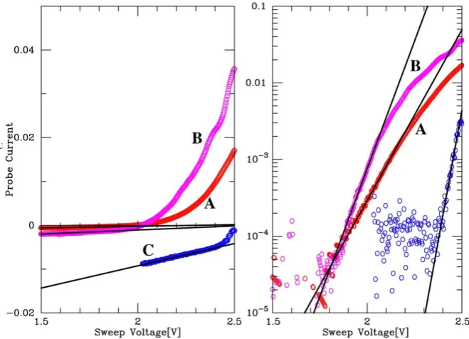
and reliability of theTe measurements, which are shown in Fig. 5. In Fig. 6a, v-i characteristic curves in the height range of 101.5–102.2 km are shown in the left part of the figure and the electron current is plotted in a logarithmic scale versus probe voltage in the right part of the figure. Comparison be-tween the v-i current characteristic curves (left) and the semi-log plotted electron current characteristic shows that the elec-tron temperature is calculated only from the very beginning of the rising part of the current-voltage characteristic curve near the floating potential. The high gain of the DC am-plifier (output voltage of 5 V for 0.01 microamperes) has a resolution of 3.9×10−5microampere. The middle gain (out-put voltage of 5 V for 0.1 microampere) has a resolution of 2.5×10−5microampere during 78–108 s; the semi-log plot-ting of the small electron current is possible, as shown in the right figure. Our observation shows that the high gain output with an 8-bit A/D converter is still acceptable.

The rocket goes into the Es layer with the order of the curves A, B, and then C. The change in the slope is clearly seen for the semi-log plotted curves.Tereduces as theNe

in-creases from A to C. We could not obtain the full v-i curve at point C, because the rocket potential went down to negative to the extent that the probe bias could not cover the volt-age range sufficiently to obtain the full v-i curve. Above the height marked C, the rocket potential further became nega-tive and therefore the v-i curve showed only an ion saturation region andTewas not available.

In Fig. 6b, three similar curves in the height range of 103.7 km to 104.4 km, where Ne decreases from the maxi-mum to the minimaxi-mum are shown. The slope of the semi-log plotted electron curve reduces from curves D to F. Te of curve F shows the highest among the three curves, which shows thatTeincreases asNedecreases.

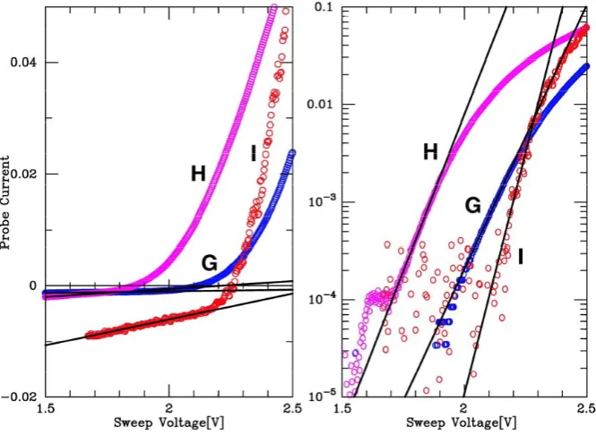
Figure 6c shows the height range from 104.4 km to 105 km, whereNestarts to increase from its minimum value toward the peak value. AlthoughTedoes not decrease on the order of the increase inNe (compare the slope of the semi-log plotted curve, G and H),Teis surely lower at higherNe. Above the heightI, the rocket potential again becomes nega-tive far below the probe sweep voltage, and the v-i curve was not available.

The mechanism of the abnormal increase in the negative potential of the rocket is not clear at this moment. However, one possible explanation could be related to the collection of the electrons/ions of the sounding rocket with the exis-tence of strong horizontal neutral wind. In fact, the rocket S-310-32 observed a strong neutral. As the turbulent shadow is formed in opposition to the wind direction, ions have dif-ficulty to be collected by the rocket surface, which faces in the opposite direction to the wind, due to the larger collision frequency between the ions and neutrals. Electrons can di-rectly hit the rocket body along the magnetic field, because at the place where the electric field is radial to the rocket axis, electron does not experience anE×Bdrift around the rocket (Rohde et al., 1993). As ions are collected only by the surface area which faces the neutral wind, the rocket will become more negative in the strong neutral wind region. The amount of the collection of the electron by a rocket body might depend on the angle between the geomagnetic field and the axis of the sounding rocket. The spin motion of the rocket is independent of the ion and electron corrections, as long as the surface condition is the same with respect to the wind direction.

Although we need complicated computer work to calcu-late the potential of the rocket body, especially in the pres-ence of strong neutral wind, the speculation above should be pursued quantitatively in the near future.

5 Concluding remarks

K.-I. Oyama et al.: Electron temperature in nighttime sporadic E layer at mid-latitude 539

18

Fig.5a. 3 v- i characteristic curves (left) and semilogarithmically plotted electron currents (right) obtained at 3 places denoted as A.B, and C in Fig.4.

Fig.6a. 3 v- i characteristic curves (left) and semilog･plotted electron currents (right) obtained at 3 heights denoted as A.B, and C which are marked in Fig.5

Fig. 6a. Three v-i characteristic curves (left) and semi-log plotted electron currents (right) obtained at 3 heights denoted as A, B, and C,

which are marked in Fig. 5.

Fig.6b. Same as Fig.6c but for E.F, and D, which are marked in Fig.5

Fig. 6b. Same as Fig. 6c but for E, F, and D, which are marked in Fig. 5.

data measured so far. From this measurement, two important findings are made. Those are:

1. Electron density varies in antiphase withTe; when elec-tron density is high, elecelec-tron temperature is low. This feature was observed most clearly insideEs, that is,Te

is lower than that of outside Es. In the highest elec-tron density region (102.1 km–103.6 km),Te seems to be close toTn. It is noted that this feature was seen in all altitude ranges in the nighttime ionosphere where no direct solar EUV exists.

540 K.-I. Oyama et al.: Electron temperature in nighttime sporadic E layer at mid-latitude

20

Fig.6c. Same as Fig.6a but for H., G, and I ,which are marked in Fig.5.

Fig. 6c. Same as Fig. 6a but for H, G, and I, which are marked in Fig. 5.

2. Te in the height range of 100–110 km is, on average, 800 K, which is still much higher than the possible range of neutral temperature (about 250 K) in this height re-gion.

We now strongly believe that some heat source is still miss-ing (Oyama and Hirao, 1980), that can elevate electron tem-perature higher than neutral temtem-perature (Oyama, 2000; Ro-hde et al., 1993), or that the current theory onTeuses incor-rect parameter values, such as suggested by Jain et al. (1981) on the electron temperature in the equatorial electrojet. Fur-ther neutral density, which we usually take from MSIS, might differ from the real one (Kurihara and Oyama, 2005). The heating of electrons by a vibrationaly excited nitrogen molecule is still one of the strong candidates (Oyama, 2000; Kurihara et al., 2003).

Acknowledgements. We express our sincere thanks to the rocket launch team of the Institute of Space and Astronautical Sci-ence/Japan, Space Exploration Agency and related institutions. We also express our sincere thanks to all related ministries for their co-operation and fishery unions for their sacrifice and understanding of the project. M. Hibino did analysis of data while he was a graduate student of University of Tokyo. The paper was completed while one of the authors (K.-I. Oyama) was at the Institute of space science, National Taiwan University.

Topical Editor M. Pinnock thanks H. S. S. Sinha and P. Mura-likrishna for their help in evaluating this paper.

References

Andreyeva, L. A., Burakov, Yu. B., Katasev, L. A., Komrakov, G. P., Nesterev, V. P., Urarov, D. B., Khryukin, V. G., and Chasovitin, Yu. K.: Rocket investigations of the ionosphere at mid-latitudes, Space Res., 11, 1043–1050, 1971.

Aubry, M., Blanc, M., Clauvel, R., Taieb, C., Bowen, P. J., Norman, K., Willmore, A. P., Sayers, S., and Wager, J. H.: Some rocket results on sporadic E., Radio Sci., 1(2), 170–177, 1966. Gleeson, L. G. and Axford, W. I.: Electron and ion temperature

vari-ations in temperate zone sporadic E layers, Planet. Space Sci., 15, 749–765, 1967.

Jain, R., Nath, N., and Setty, C. S. G. K.: On Joule heating of the equatorial electrojet E-region, J. Atmos. Terr. Phys., 43, 1189– 1197, 1981.

Kurihara, J., Oyama, K.-I., Suzuki, K., and Iwagami, N.: Vibra-tional rotaVibra-tional temperature measurement of N2 in the lower thermosphere by the rocket experiment, Adv. Space Res., 32(5), 725–729, 2003.

Kurihara, J. and Oyama, K.-I.: Rocket-borne instrument for measuring vibrational-rotational temperature and density in the lower thermosphere, Rev. Sci. Instr., 76, 083101, doi:10.1063/1.1988189, 2005.

Oya, H.: Development of gyro-plasma probe, Small Rocket Instru-mentation Techniques, North Holland Publish Company, Ams-terdam, 36–47, 1969.

Oyama, K.-I.: A systematic study of several phenomena associated with contaminated Langmuir probes, Planet. Space Sci., 24, 87– 89, 1976.

Oyama, K.-I. and Hirao, K.: Application of a glass sealed Lang-muir probe to ionospheric study, Rev. Sci. Instrum., 47, 101–107, 1976.

K.-I. Oyama et al.: Electron temperature in nighttime sporadic E layer at mid-latitude 541

to 120 Km?, Planet. Space Sci., 28, 207–211, 1980.

Oyama, K.-I.: Insitu measurements ofTein the lower ionosphere – A review, Adv. Space Res., 26(8), 1231–1240, 2000.

Rohde, V., Piel, A., Thiemann, H., and Oyama, K.- I.: Insitu Diag-nostics of ionospheric plasma with the resonance cone technique, J. Geophys. Res., 98(A11), 19 163–19 172, 1993.

Schutz, S. R. and Smith, L. G.: Electron temperature measurements in the Mid-Latitude Sporadic E layers, J. Geophys. Res., 81(19), 3214–3220, 1976.

Szuszczewicz, E. P. and Holmes, J. C.: Observations of electron temperature gradients in Mid-LatitudeEs layers, J. Geophys. Res., 82(32), 5073–5080, 1977.