© European Geosciences Union 2007
Geophysicae
Quiet-condition variations in the scale height at F2-layer peak at
Jicamarca during solar minimum and maximum
C.-C. Lee1and B. W. Reinisch2
1General Education Center, Ching-Yun University, Jhongli City, Taoyuan County, Taiwan 2Center for Atmospheric Research, University of Massachusetts, Lowell, Massachusetts, USA
Received: 13 August 2007 – Revised: 16 November 2007 – Accepted: 4 December 2007 – Published: 2 January 2008
Abstract. This study is the first attempt to examine the quiet-condition variations in scale height (Hm) near the F2-layer peak in the equatorial ionosphere. The data periods of Hm derived from the Jicamarca ionograms are January-December 1996 and April 1999–March 2000. The results show that the greatest and smallest Hm values are generally at 11:00–12:00 LT and 04:00–05:00 LT, respectively. Addi-tionally, the sunrise peak occurs at 06:00 LT only during solar minimum. The post-sunset peaks in the equinoctial and sum-mer months are more obvious during solar maximum. The Hm difference between solar minimum and maximum are significant from afternoon to midnight. On the other hand, the Hm values during 07:00–10:00 LT for solar minimum are close to those for solar maximum. Furthermore, the cor-relation of Hm with the critical frequency (foF2) of F2-layer is generally low. In contrast, the correlation between Hm and the peak height (hmF2) of F2-layer is high. For Hm and the thickness parameter (B0) of F2-layer, the correlation be-tween these two parameters is almost perfect.
Keywords. Ionosphere (Equatorial ionosphere; Modeling and forecasting)
1 Introduction
The understanding of the electron density profile, which is the altitude distribution of electron density, is important for the ionospheric studies. In general, the electron density pro-file of the bottomside ionosphere is provided by the measure-ments of ground-based digisonde/ionosonde (e.g. Reinisch, 1996) or by incoherent scatter radar (ISR) (e.g. Liu et al, 2007). For the topside ionosphere, the profile can be obtained from the ISR, the space-born instruments (e.g. Stankov et al., 2006), or by analytic functions. In the past decades, many Correspondence to: C.-C. Lee
analytic functions, such as Chapman, exponential, parabolic, and sech-squared functions, have been applied to depict the ionospheric profile (e.g. Booker, 1977; Rawer et al., 1985; Rawer, 1988; Di Giovanni and Radicella, 1990; Huang and Reinisch, 2001; Stankov et al., 2003). In these analytic func-tions, in addition to the density and height of F2-layer peak, the scale height is an important parameter to describe the ionospheric profile.
In Huang and Reinisch (2001) and Reinisch and Huang (2001), a new technique was introduced to derive the scale height (Hm) near the F2-layer peak from the shape of the bottomside profile. Then, Reinisch et al. (2004) showed that the Hm can help to improve the model of topside profile in International Reference Ionosphere (IRI) (Bilitza, 2001). Recently, the diurnal, seasonal, and solar activity variations of Hm at Wuhan (30.6◦N, 114.4◦E) and the yearly varia-tion of Hm of Wuhan and 12 other stavaria-tions were investigated by Liu et al. (2006). The diurnal and seasonal variations of Hm at Hainan (19.4◦N, 109.0◦E) and two European stations were studied by Zhang et al. (2006) and Mosert et al. (2007), respectively. The Hm values were compared with the top-side scale height of toptop-side sounders model by Belehaki et al. (2006). Till now, the Hm near the dip equator has not been examined, although many studies of Hm have been done.
In the present work, the Hm values obtained from the equatorial ionograms recorded by the Jicamarca digisonde (12◦S, 76.9◦W, dip latitude: 1.0◦N) during geomagnetic quiet-conditions are examined. The correlations of Hm with the critical frequency (foF2), peak height (hmF2), and thick-ness parameter (B0) of F2-layer are also analyzed here.
2 Data analysis
2542 C.-C. Lee and B. W. Reinisch: Quiet-condition variations in the scale height
Table 1. The monthly smoothed sunspot numbers (SSN) for January-December 1996 and April 1999–March 2000.
Month Monthly Month Monthly (solar minimum) SSN (solar maximum) SSN January 1996 10.4 January 2000 112.9 February 1996 10.1 February 2000 116.8 March 1996 9.7 March 2000 119.9 April 1996 8.4 April 1999 85.5 May 1996 8.0 May 1999 90.5 June 1996 8.5 June 1999 93.1 July 1996 8.4 July 1999 94.3 August 1996 8.3 August 1999 97.5 September 1996 8.4 September 1999 102.3 October 1996 8.8 October 1999 107.8 November 1996 9.8 November 1999 111.0 December 1996 10.4 December 1999 111.1
1996 and April 1999–March 2000. It is noted the solar cycle 23 started in May 1996 with the monthly smoothed sunspot number (SSN) at 8.0 and peaked in April 2000 at 120.8. The SSN of these 24 months are displayed in Table 1. There-fore, the period of January-December 1996 is categorized to the solar minimum; while the April 1999–March 2000 is at-tributed to the solar maximum.
The Jicamarca ionograms were downloaded from the Digital Ionogram DataBase (DIDBase). foF2 is ob-tained from the ionograms using the SAO-Explorer soft-ware package (http://ulcar.uml.edu/digisonde.html). The values of hmF2, B0, and Hm were derived using the true height inversion algorithm NHPC (ftp://umlcar.uml. edu/SoftwareUtilities/NHPC/) (Reinisch and Huang, 1998; Huang and Reinisch, 2001) imbedded in the SAO-Explorer. In order to eliminate possible effects of geomagnetic disturbed-condition, the data of those days for geomagnetic quiet-conditions are applied in the following analyses. No-tice that the geomagnetic quiet-condition means the sum of the eightKpindices for the day is less than or equal to 24 (6Kp≤24).
3 Results and discussion
3.1 Diurnal and seasonal variations of Hm
Figure 1 illustrates the monthly median values of Hm for the equinoctial (March–April and September–October 1996), summer (May, June, July, and August 1996), and winter (January–February and November–December 1996) months during solar minimum. In the equinoctial months (Fig. 1a), the Hm values exhibit a clear diurnal variation. The great-est and smallgreat-est values occur at 05:00 and 12:00 LT, respec-tively. This diurnal variation is understandable from the
clas-Fig. 1. The quiet-condition monthly median values of Hm for the (a) equinoctial, (b) summer, and (c) winter months during January–
December 1996.
[image:2.595.50.284.97.266.2]Fig. 2. The quiet-condition monthly median values of Hm for the (a) equinoctial, (b) summer, and (c) winter months during April
1999–March 2000.
two peaks might not be produced by an increasing tempera-ture, but by the shape change of the electron density profile. In the sunrise period, the shape change of electron profile due to the solar production at higher altitudes would form an increase of hmF2 and B0 (Lee et al., 2007). Further, this kind of change could cause a sunrise peak of Hm. During the post-sunset period, the pre-reversal enhancement (PRE)
Fig. 3. The difference (1Hm) of monthly median Hm between so-lar minimum and maximum. Notice that the1Hm is obtained by subtracting the monthly median Hm for solar maximum from that for solar minimum.
ofE×Bdrift velocity (Farley et al., 1986) would make the post-sunset peaks of hmF2 and B0 (Lee and Reinisch, 2006; Lee et al., 2007), and in turn form a post-sunset peak in Hm. In Fig. 1b, the diurnal variations of Hm in the summer months are similar to those in the equinoctial months, ex-cept November. For January, February, and December, the greatest and smallest values of Hm are at 04:00–05:00 LT and 11:00–12:00 LT, respectively. For November, the day-time variation of Hm is different from those observed in the three other months. Based on the results for hmF2 and B0 in November 1996 (Lee et al., 2007), this different daytime variation in Hm is caused by the variation in the vertical ve-locity. Furthermore, in this season, the post-sunset peak curs at different time for each month. These different oc-curring times of post-sunset peaks are related to the different behaviors of the PREE×B drift velocity, which also pro-duce the different times of the hmF2 and B0 peaks in the post-sunset period (Lee et al., 2007).
In the winter months (Fig. 1c), the diurnal variations are generally similar to those observed in two other seasons. It is noted that the maximum Hm values at 12:00 LT in this season are larger than those observed in the equinoctial and summer months. In winter, the B0 values are larger than those observed in other seasons (Lee et al., 2007). Therefore, the larger Hm values would be related to the larger B0 values in this season, because Hm is highly correlated to B0 (see Sect. 3.2). Moreover, the post-sunset peak does not appear, because the PREE×B drift velocity is not obvious in this season (Fejer et al., 1999; Lee et al., 2007).
[image:3.595.88.244.67.553.2]2544 C.-C. Lee and B. W. Reinisch: Quiet-condition variations in the scale height
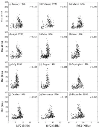
Fig. 4. The scatter plots of Hm versus foF2 during January–December 1996. The correlation coefficient (r) of Hm and foF2 is placed in the upper-right corner.
and October 1999), summer (May, June, July, and August, 1999), and winter (January–February 2000 and November– December 1999) months are displayed in Fig. 2. In Fig. 2a, the occurring times for the greatest (12:00–13:00 LT) and smallest (05:00–06:00 LT) values are generally close to those for solar minimum. However, two significant differences are found between solar minimum and maximum. One is that the sunrise Hm peak does not exist during solar maximum. This absent sunrise peak indicates that the effect of solar pro-duction at higher altitudes on the profile change does not appear during solar maximum. The other difference is that the Hm values have a larger post-sunset peak during solar maximum. According to Fejer et al. (1999), this larger
Fig. 5. The scatter plots of Hm versus foF2 during April 1999–March 2000. The correlation coefficient (r) of Hm and foF2 is placed in the upper-right corner.
Figure 3 shows the1Hm values where1Hm is the dif-ference of the monthly median values of Hm during solar minimum and the corresponding median values during solar maximum. The significantly negative1Hm from afternoon to midnight demonstrate that the Hm for solar maximum is obviously larger than that observed for solar minimum dur-ing this time period. Furthermore, the positive differences at noon in the winter months indicate that the noontime Hm for this season is larger during solar minimum. In contrast, the negative differences at noon in the equinoctial and summer months reveal that the noontime Hm is smaller for these two seasons during solar minimum. In addition, the Hm values during 07:00–10:00 LT of solar minimum and maximum are
close. This similarity indicates that the Hm values during 07:00–10:00 LT are not varied by the solar activity.
3.2 Correlations of Hm with foF2, hmF2, and B0
2546 C.-C. Lee and B. W. Reinisch: Quiet-condition variations in the scale height
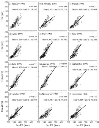
Fig. 6. The scatter plots of Hm versus hmF2 during January–December 1996. The correlation coefficient (r) of Hm and hmF2 and the equation of least-squares straight line (solid line) for each month are placed in the upper-right corner.
maximum (Fig. 5), the correlation between Hm and foF2 is better than during solar minimum. The correlation coeffi-cients range between 0.221 and 0.410 in summer, between 0.464 and 0.50 in equinox, and between 0.580 and 0.635 in winter. These results near the dip equator are not the totally same as those observed at other latitudes. At low-latitude, Liu et al. (2006) showed that a weak negative or poor cor-relation exists between Hm and foF2 at Wuhan (30.6◦N, 114.4◦E). The poor correlation was also found Zhang et al. (2006) using data from the low-latitude station, Hainan (19.4◦N, 109.0◦E). The largerrvalues at Jicamarca demon-strate that the correlation between Hm and foF2 in the equa-torial ionosphere is higher than those at other latitudes.
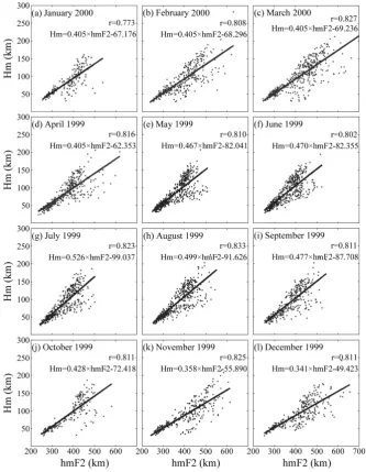
Fig. 7. The scatter plots of Hm versus hmF2 during April 1999–March 2000. The correlation coefficient (r) of Hm and hmF2 and the equation of least-squares straight line (solid line) for each month are placed in the upper-right corner.
maximum. In August 1996 (Fig. 6h), ther value is 0.890 and the straight line is given as Hm=0.869×hmF2-189.458. In August 1999 (Fig. 7h), thervalue is 0.833 and the straight line is given as Hm=0.499×hmF2-91.626. In addition, ther
values of the equinoctial and winter months are larger during solar minimum than during solar maximum. On the other hand, thervalues of the summer months are smaller during solar minimum than during solar maximum.
The high correlation between Hm and hmF2 (r=0.700– 0.890) demonstrate that the physical processes controlling the hmF2 variations might also be responsible for the Hm variations. In the equatorial ionosphere, the hmF2 variation mainly depends on the verticalE×Bvelocity because of the
horizontal geomagnetic field line (Lee and Reinisch, 2006; Lee et al., 2007). Therefore, the Hm variation near the dip equator would be also affected by the verticalE×Bvelocity. Moreover, thervalues in this study are larger than those in Liu et al. (2006) and Zhang et al. (2006). This suggests that dependence of Hm on hmF2 is more obvious near the dip equator than at low-latitudes.
2548 C.-C. Lee and B. W. Reinisch: Quiet-condition variations in the scale height
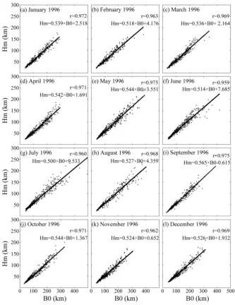
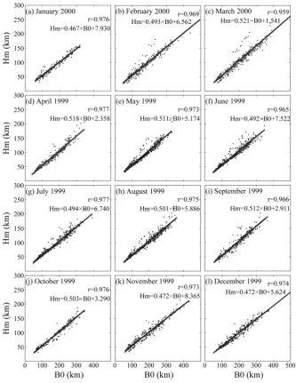
Fig. 8. The scatter plots of Hm versus B0 during January–December 1996. The correlation coefficient (r) of Hm and B0 and the equation of least-squares straight line (solid line) for each month are placed in the upper-right corner.
found at low-latitudes (Liu et al., 2006; Zhang et al., 2006). These results indicate that the Hm values in the equatorial ionosphere can be estimated from the B0 values, based on the equations of least-squares straight lines in Figs. 8 and 9. For the ionospheric model, especially for IRI-2001 (Bilitza, 2001), the electron profile of topside ionosphere can be de-rived from the B0 parameter.
4 Summary
In this study, we analyze for the first time, the diurnal and seasonal variations of the scale height (Hm) at F2-layer peak
near the dip equator during the solar minimum and maxi-mum. The Hm values are derived from the Jicamarca iono-grams from January to December 1996 and from April 1999 to March 2000. To eliminate the effects of geomagnetic dis-turbances, only the data under quiet-conditions are used in the study. The correlations of Hm with foF2, hmF2 and B0 are also calculated.
Fig. 9. The scatter plots of Hm versus B0 during April 1999–March 2000. The correlation coefficient (r) of Hm and B0 and the equation of least-squares straight line (solid line) for each month are placed in the upper-right corner.
months, the post-sunset peak is absent for both solar mini-mum and maximini-mum. During solar minimini-mum, the maximini-mum Hm values at noon are greater in the winter months. Dur-ing solar maximum, the maximum Hm values at noon are greater in the equinoctial and winter months. The Hm differ-ences are significant from afternoon to midnight. In contrast, the Hm values of solar minimum and maximum are close to each other during 07:00–10:00 LT.
The correlation coefficients between Hm and foF2 are less than 0.40 during 9 months of the low solar activity year and during 3 months of the high solar activity period. The moder-ate correlations (r=0.402–0.580) appear in 3 months of solar minimum and 6 months of solar maximum. Only 3 months
2550 C.-C. Lee and B. W. Reinisch: Quiet-condition variations in the scale height
Acknowledgements. CCL was supported by the grant of National
Science Council NSC 96-2119-M-231-001. BWR was supported by the AF grant #FA8718-06-C-0072. The authors would like to thank UML for access to DIDBase (http://ulcar.uml.edu/DIDBase/), and to the National Geophysical Data Center (NGDC) (http://www. ngdc.noaa.gov/) for providing data ofKpand sunspot number. The authors thank the two referees for the valuable comments and sug-gestions.
Topical Editor M. Pinnock thanks two anonymous referees for their help in evaluating this paper.
References
Belehaki, A., Marinov, P., Kutiev, I., Jakowski, N., and Stankov, S.: Comparison of the topside ionosphere scale height determined by topside sounders model and bottomside digisonde profile, Adv. Space Res., 37, 963–966, 2006.
Bilitza, D.: International Reference ionosphere 2000, Radio Sci., 36, 261–275, 2001.
Booker, H. G.: Fitting of multi-region ionospheric profiles of elec-tron density by a single analytic function of height, J. Atmos. Terr. Phys., 39, 619–623, 1977.
Di Giovanni, G. and Radicella, S. M.: An analytical model of the electron density profile in the ionosphere, Adv. Space Res., 10(11), 27–30, 1990.
Farley, D. T., Bonelli, E., and Fejer, B. G..: The pre-reversal en-hancement of the zonal electric field in the equatorial ionosphere. J. Geophys. Res., 91, 13 723–13 728, 1986.
Fejer, B. G., de Paula, E. R., Gonzales, S. A., and Woodman, R. F.: Average vertical and zonal plasma drift over Jicamarca, J. Geophys. Res., 96, 13 901–13 906, 1991.
Fejer, B. G., Scherliess, L., and de Paula, E. R.: Effects of the verti-cal plasma drift velocity on the generation and evolution of equa-torial F, J. Geophys. Res., 104, 19 859–19 869, 1999.
Huang, X. and Reinisch, B. W.: Vertical electron content from iono-gram in real time, Radio Sci., 36, 335–342, 2001.
Lee, C. C. and Reinisch, B. W.: Quiet-condition hmF2, NmF2, and B0 variations at Jicamarca and comparison with IRI-2001 during solar maximum, J. Atmos. Sol.-Terr. Phy., 68, 18, 2138–2146, 2006.
Lee, C. C., Reinisch, B. W., Su, S. -Y., and Chen, W. S.: Quiet-time variations of F2 layer parameters at Jicamarca and comparison with IRI-2001 during solar minimum, J. Atmos. Sol-Terr. Phy., in press, 2007.
Liu, L., Wan, W., and Ning, B.: A study of the ionogram derived effective scale height around the ionospheric hmF2, Ann. Geo-phys., 24, 851–860, 2006,
http://www.ann-geophys.net/24/851/2006/.
Liu, L., Le, H., Wan, W., Sulzer, M. P., Lei, J. and Zhang, M. L.: An analysis of the scale height in the lower topside ionosphere based on the Arecibo incoherent scatter radar measurements, J. Geophys. Res., 112, A06307, doi:10.1029/2007JA012250, 2007. Mosert, M., Ezquer, R., de la Morene, B., Altadill, D., Mansilla, G., and Miro Amarante, G.: Behaviors of the scale height at the Fe layer peak derived from digisonde measurements at tow Eu-ropean stations, Adv. Space Res., 39, 755–758, 2007.
Rawer, K.: Synthesis of ionospheric electron density profiles with Epstein functions, Adv. Space Res., 8(4), 191–198, 1988. Rawer, K., Bilitza, D., and Gulyaeva, T. L.: New formulas for IRI
electron density profile in the topside and middle ionosphere, Adv. Space Res., 5(7), 3–12, 1985.
Reinisch, B. W.: Modern ionosondes, in Modern Radio Science, edited by: Kohl, H., Ruester, R., and Schlegel, K., European Geophysical Society, Katlenburg-Lindau, Germany, 440–458, 1996.
Reinisch, B. W. and Huang, X.: Finding better B0 and B1 param-eters for the IRI F2 profile function, Adv. Space Res., 22, 741– 747, 1998
Reinisch, B. W. and Huang, X.: Deducing topside profile and total electron content form bottomside ionograms, Adv. Space Res., 27(1), 23–30, 2001.
Reinisch, B. W., Huang, X. Q., Belehaki, A., Shi, J. H., Zhang, M. L., and Iima, R.: Modeling the IRI topside profile using scale heights from ground-based ionosonde measurements, Adv. Space Res., 34(9), 2026–2031, 2004.
Stankov, S. M. and Jakowski, N.: Topside plasma scale height re-trieved from radio occultation measurements, Adv. Space Res., 37, 958–962, 2006.
Stankov, S. M., Jakowski, N., Heise, S., Muhtarov, P., Ku-tiev, I., and Warnant, R.: A new method for reconstruction of the vertical electron density distribution in the upper iono-sphere and plasmaiono-sphere, J. Geophys. Res., 108(A5), 1164, doi:10.1029/2002JA009570, 2003.