NORMALIZATION
So Now what is Normalization?
GOLDEN RULE OF NORMALIZATION:
Enter The Minimum Data Necessary, Avoiding Duplicate Entry Of Information, With
Minimum Risks To DataIntegrity.
Goals Of Normalization:
Eliminate Redundancies Caused By:
Fields Repeated Within A File
Fields Not Directly Describing The Key Entity Fields Derived From Other Fields
Avoid Anomalies In Updating (Adding, Editing,Deleting)
Represent Accurately The Items Being Modeled
Definition
Normalization
is a process for assigning attributes to entities. It
reduces data redundancies and helps eliminate the data anomalies.
Normalization works through a series of stages called normal forms:
First normal form (1NF)
Second normal form (2NF)
Third normal form (3NF)
Basic Rule for Normalization
The attribute values in a relational table should be functionally
dependent (FD) on the primary key value.
A relationship is functionally dependent when one attribute value implies or
determines the attribute value for the other attribute.
EM_SS_NUM --> EM_NAME
Corollaries
Corollary 1:
No repeating groups allowed in relational tables.
Benefits
Facilitates data integration. Reduces data redundancy.
Provides a robust architecture for retrieving and maintaining data.
Compliments data modelling.
First Normal Form
Disallows composite attributes, multivalued attributes, and nested relations; attributes whose values for an individual tuple are non-atomic
Considered to be part of the definition of relation
6
Figure 10.8 Normalization into 1NF
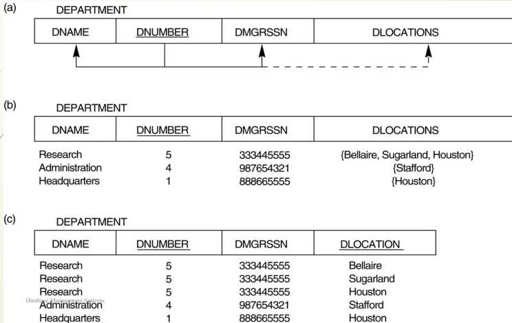
FIGURE 10.9
Normalizing nested
relations into 1NF.
(a) Schema of the EMP_PROJ relation with a “nested relation” attribute PROJS. (b) Example extension of the EMP_PROJ relation showing nestedrelations within each tuple. (c) Decomposition of EMP_PROJ into relations EMP_PROJ1 and EMP_PROJ2 by propagating the primary key.
8
Second Normal Form (1)
Uses the concepts of
FD
s,
primary key
Definitions:
Prime attribute
- attribute that is member of the
primary key K
Full functional dependency
- a FD Y
->
Z where
removal of any attribute from Y means the FD does
not hold any more
Examples:
- {SSN, PNUMBER}
->
HOURS is a full FD since
neither SSN
->
HOURS nor PNUMBER
->
HOURS hold
- {SSN, PNUMBER}
->
ENAME is
not
a full FD (it is called a
partial dependency
) since SSN
->
ENAME also holds
Second Normal Form (2)
A relation schema R is in
second normal form
(
2NF
) if every non-prime attribute
A in R is fully functionally dependent on the primary key
R can be decomposed into 2NF relations via the process of 2NF normalization
10
FIGURE 10.3
FIGURE 10.10
Normalizing into 2NF and 3NF.
(a) Normalizing EMP_PROJ into 2NF relations
12
Third Normal Form
(1)
Definition:
Transitive functional dependency
-
a FD X
->
Z that can be derived
from two FDs X
->
Y and Y
->
Z
Examples:
-
SSN
->
DMGRSSN is a
transitive
FD since
SSN
->
DNUMBER and DNUMBER
->
DMGRSSN hold
- SSN
->
ENAME is
non-transitive
since there is no set of attributes X where
SSN
->
X and X
->
ENAME
Third Normal Form
(2)
A relation schema R is in
third normal form
(
3NF
) if it is
in 2NF
and
no non-prime attribute A in R is transitively
dependent on the primary key
R can be decomposed into 3NF relations via the process of
3NF normalization
NOTE:
In
X
->
Y and Y
->
Z, with X as the primary key, we consider this a problem
only if Y is not a candidate key. When Y is a candidate key, there is no problem
with the transitive dependency .
E.g., Consider EMP (SSN, Emp#, Salary ).
Here, SSN
->
Emp#
->
Salary and Emp# is a candidate key.
14
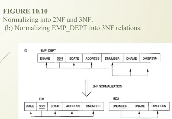
FIGURE 10.10
Normalizing into 2NF and 3NF.
(b) Normalizing EMP_DEPT into 3NF relations.
16
General Normal Form Definitions (For
Multiple Keys)
The above definitions consider the primary key only
The following more general definitions take into account
relations with multiple candidate keys
General Definition of Second Normal Form
A relation schema R is in second normal form (2NF) if every nonprime attribute A in R is not partially dependent on any key of R.
18
FIGURE 10.11
Normalization into 2NF
(a) the LOTS relation with its functional dependencies FD1 though FD4. (b) Decomposing into the 2NF relations LOTS1 and LOTS2.General Definition of Third Normal Form
Definition:
Superkey
of relation schema R - a set of attributes S of R that
contains a key of R
A relation schema R is in
third normal form
(
3NF
) if
whenever a FD X
->
A holds in R, then either:
(a) X is a superkey of R, or
(b) A is a prime attribute of R
NOTE:
Boyce-Codd normal form disallows condition (b) above
20
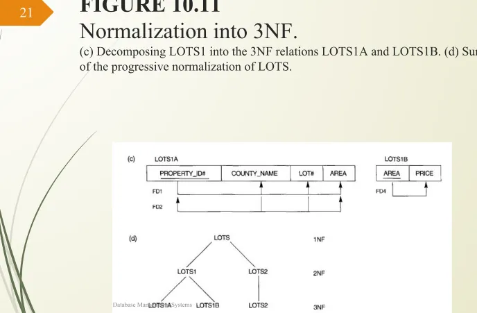
FIGURE 10.11
Normalization into 3NF.
(c) Decomposing LOTS1 into the 3NF relations LOTS1A and LOTS1B. (d) Summary of the progressive normalization of LOTS.
BCNF (Boyce-Codd Normal Form)
A relation schema R is in
Boyce-Codd Normal Form
(
BCNF
)
if whenever an FD X
->
A holds in R, then X is a superkey of
R
Each normal form is strictly stronger than the previous one
Every 2NF relation is in 1NF
Every 3NF relation is in 2NF
Every BCNF relation is in 3NF
There exist relations that are in 3NF but not in BCNF
The goal is to have each relation in BCNF (or 3NF)
22
FIGURE 10.12
Boyce-Codd normal form.
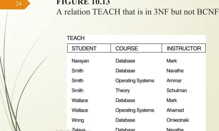
(a) BCNF normalization of LOTS1A with the functional dependency FD2 being lost in the decomposition. (b) A schematic relation with FDs; it is in 3NF, but not in BCNF.FIGURE 10.13
A relation TEACH that is in 3NF but not BCNF.
24
Achieving the BCNF by Decomposition (1)
Two FDs exist in the relation TEACH:
fd1: { student, course} -> instructor
fd2: instructor ->
course
{student, course} is a candidate key for this relation and that the
dependencies shown follow the pattern in Figure 10.12 (b). So this
relation is in 3NF but not in BCNF
A relation
NOT
in BCNF should be decomposed so as to meet this
property, while possibly forgoing the preservation of all functional
dependencies in the decomposed relations. (See Algorithm 11.3)
Achieving the BCNF by Decomposition (2)
Three possible decompositions for relation TEACH
1. {student, instructor} and {student, course}
2. {course, instructor } and {course, student}
3. {instructor, course } and {instructor, student}
All three decompositions will lose fd1. We have to settle for sacrificing the functional dependency preservation. But we cannot sacrifice the non-additivity property after decomposition.
Out of the above three, only the 3rd decomposition will not generate spurious tuples after join.(and hence has the non-additivity property).
A test to determine whether a binary decomposition (decomposition into two relations) is nonadditive (lossless) is discussed in section 11.1.4 under Property LJ1. Verify that the third decomposition above meets the property.