PONR carp final JAEREform

(1)

Opposing irreversibilities and tipping point uncertainty

Charles Sims ([email protected]), Faculty Fellow at the Howard H. Baker Jr. Center for Public Policy and an assistant professor in the Department of Economics at the University of Tennessee, 1640 Cumberland Ave, Knoxville, TN 37920.

David Finnoff ([email protected]), Associate professor in the Department of Economics and Finance, 1000 E. University Avenue, University of Wyoming, Laramie, WY 82071.

Abstract: Irreversible environmental damage can lead to a more “conservationist” policy than would otherwise be optimal while sunk costs and policy persistence create an economic

irreversibility that leads to policies that are less “conservationist” than they otherwise would be. The economic irreversibility effect is often larger than the irreversibility associated with

environmental damage. We revisit this result in a novel context with multiple uncertainties and an avoidable tipping point which triggers irreversible damage. An optimal stopping model over dynamic environmental lotteries is developed to characterize the optimal timing and stringency of an environmental policy subject to two kinds of irreversibility (economic and an

environmental tipping point), two tipping point mechanisms (critical damage thresholds and random events), and two kinds of uncertainty (uncertain system dynamics and uncertainty in when the tipping point will be crossed). Using an example of Asian carp invasion into Lake Michigan, results illustrate how differing definitions of precautionary behavior and beliefs about the degree of environmental irreversibility may help explain persistent debates in environmental policy.

Keywords: tipping point; catastrophic event; option value; uncertainty; invasive species

(2)

2 Introduction

Most debates over environmental risk reduction policies boil down to a question of how much society should invest in the policy and when society ought to invest. For example, the relatively certain cost burden associated with reducing the possibility of irreversible climate change pits proponents of stringent and early risk mitigation (Stern 2007) against advocates of a more incremental and gradual approach (Nordhaus 2014). Similarly, the threat of damage from a permanently established bioinvader pits supporters of costly eradication strategies (Simberloff 2011) against proponents of a “wait and see” approach, attempting to discern which species will actually become problematic (Davis et al. 2011). The answers depend on a tension between the threat of irreversible environmental damage and the certainty of economic irreversibilities such as sunk costs and transaction costs that lead to policy persistence (Coate and Morris 1999; Zhao and Kling 2003). Arguments for early and stringent action focus on the sunk benefits of a policy when it reduces the risk of an irreversible transformation of the environment (Farzin 1996). For example, adoption of abatement technologies or cap-and trade policies that lessen additions to a stock pollutant provide benefits far into the future. But, these sunk benefits are often dominated by the sunk costs and policy persistence associated with these actions (Fisher and Narain 2003; Kolstad 1996; Nordhaus 1994; Pindyck 2000, 2002; Saphores 2004; Wirl 2006), providing a behavioral basis for delay.1

However, for many of the key environmental problems facing societies, the environmental damages are thought to be characterized by tipping points, beyond which

significant irreversible environmental damage is incurred (Crépin et al. 2012; Horan et al. 2011).

1

(3)

3

These tipping points add an additional dimension to the irreversibility, in that investments that were once effective become ineffective. In addition, there is often little known about where these tipping points are located, or how big a change is necessary before the tipping point is crossed. Unknown tipping points suggest a reduction in the value of delaying risk reduction policies since the option to act may unexpectedly expire. However, it remains unresolved as to whether the presence of an unknown tipping point can overwhelm the value in delaying sunk costs and policy persistence and provide a justification for more precautionary behavior (Carpenter, Ludwig and Brock 1999; Clarke and Reed 1994; Iovanna and Newbold 2007; Ludwig, Carpenter and Brock 2003; Saphores 2003; Tsur and Zemel 1996). The dominant opportunity costs from sunk costs or irreversible commitments results in an option value that must be balanced against the opportunity cost of delaying action – unexpectedly reaching a tipping point that subjects society to irreversible environmental damage.

We develop a theoretical model that characterizes the optimal timing and stringency of an environmental policy subject to two kinds of irreversibility (economic and an environmental tipping point), two tipping point mechanisms (critical damage thresholds and random events), and two kinds of uncertainty (uncertain system dynamics and uncertainty in when the tipping point will be crossed). We demonstrate that while an unknown tipping point does reduce the value of delaying an irreversible investment,2 it is not enough to extinguish the value of delay. We find that regardless of whether the tipping point is triggered by random events (Clarke and Reed 1994; Zemel 2012) or triggered by crossing an unknown threshold in the state space (Nævdal 2003, 2006; Tsur and Zemel 1996) there remains value in delaying an investment that lessens environmental damage, yet less than if there were no tipping point.

2_{Specifically, if economic activity causes an irreversible transformation of the environment, the expected net}

(4)

4

The results are demonstrated in a specific context of Asian carp invasion into the Great Lakes. The invasion is thought to immediately threaten Lake Michigan’s large recreational fishery, yet whether Asian carp have already established in Lake Michigan has been the source of a fierce debate (Wines 2014). If the carp have already established, then a proposed (costly) hydro-separation of the Mississippi and Great Lakes watersheds would be ineffective. If establishment has not yet occurred, hydro-separation may work in avoiding the invasion. Proponents of hydro-separation cite the possibility of avoiding irreversible environmental damage caused by Asian carp establishment while opponents cite the large sunk costs associated with the project and the possibility that establishment may have already occurred. We use the model to weigh the relative merits of both arguments.

The model and its insights are applicable to a wide range of environmental policies in response to unknown environmental tipping points. For example, the melting of ice sheets is thought to be unstoppable once a temperature tipping point is crossed (Lenton et al. 2008). The problem is that the location of these tipping points can only be pinpointed probabilistically (Robinson, Calov and Ganopolski 2012). Likewise, it is commonly thought that wildlife species are subject to minimum viable populations, below which the species will go extinct. However, the lack of data at low population levels makes it difficult to identify this critical population with any certainty (Reed et al. 2003). Model insights could also be applied more generally to

(5)

5

The following section develops a model of investment in damage mitigation within a system subject to stochastic shocks and an unexpected, irreversible tipping point that reduces the efficacy of the investment. Section three describes how the dynamically optimal mitigation investment is akin to a choice between stochastic dynamic environmental lotteries. Section four applies the model to the Asian carp case study. Section five concludes and discusses avenues for future work.

2. Opposing irreversibilities and tipping point uncertainty

Consider a system where economic activity creates a stock of pollution that causes a flow of environmental damage 𝐷(𝑡). Examples include pollution created from manufacturing,

invasive species introduced through trade, or habitat loss from agricultural conversion and deforestation. Future damage evolves according to a generalized Ito process 𝑑𝐷 = 𝛼₀(𝐷)𝑑𝑡 + 𝜎₀(𝐷)𝑑𝑧 where 𝛼₀(𝐷) > 0 is the (possibly) non-constant growth in damage absent any control, 𝜎02(𝐷) is the instantaneous variance parameter, and dz is the increment of a standard Wiener process.3 Larger values for 𝛼0 imply more rapid environmental degradation corresponding to a more mobile pest species, expedient fate and transport of pollutants, or contagious disease. Larger values of 𝜎₀ correspond to a larger amount of uncertainty in future damages.

If the tipping point has not been crossed, the resource manager can mitigate the environmental degradation by investing in a policy that instantly reduces the trend in damage from 𝛼₀(𝐷) to 𝛼₁(𝐷) and possibly the variance from 𝜎₀(𝐷) to 𝜎₁(𝐷) for all D. A strategy which results in 𝛼₁(𝐷) < 0 will permanently reverse the increasing trend in damages, 0 < 𝛼₁(𝐷) <

3_{This flexible specification can accommodate many popular stochastic processes such as arithmetic Brownian}

motion (𝛼0(𝐷) = 𝛼0; 𝜎0(𝐷) = 𝜎0), geometric Brownian motion (𝛼0(𝐷) = 𝛼0𝐷; 𝜎0(𝐷) = 𝜎0𝐷), and an

(6)

6

𝛼0(𝐷) slows damages, and a razor’s edge strategy (𝛼1(𝐷) = 0) assumes damages randomly evolve with no trend. A strategy which results in 𝜎1(𝐷) < 𝜎0(𝐷) reflects less volatility in future damage. Adopting this policy would impose an irreversible flow of sunk costs on society – an economic irreversibility. For instance, a strategy aimed at controlling pollution emissions may require emitting firms to alter their production process or invest in end-of-pipe technologies. An invasive species control strategy may prohibit trade in commodities known to harbor invasives. The present value of the flow of sunk cost associated with this strategy at time of implementation is a function of the stringency of the strategy: 𝐶(𝐷) = 𝑐_𝛼[𝛼₀(𝐷) − 𝛼₁(𝐷)]2+ 𝑐_𝜎[𝜎₀(𝐷) − 𝜎1(𝐷)]2 where 𝑐𝛼 > 0 and 𝑐𝜎 > 0.

There is also an opportunity cost of adopting the strategy immediately since sunk costs limit the ability to respond to new information. For example, a decision maker may regret implementing the policy since environmentally-favorable shocks may cause damages to be smaller than initially thought and the costs cannot be recouped. This opportunity cost is known as an option value and arises when sunk costs or irreversible commitments are required to secure an uncertain stream of benefits (Dixit and Pindyck 1994).4

However, this option value must be balanced against the opportunity cost of delaying action – unexpectedly reaching a tipping point that results in the manager being unable to mitigate environmental damage. Economic studies often distinguish between reversible thresholds which allow for regeneration or healing (Brozović and Schlenker 2011; Tsur and Zemel 1998, 2004) and irreversible thresholds where damage is permanent (Keller, Bolker and Bradford 2004; Nævdal 2006; Tsur and Zemel 1995). Our concept of an irreversible tipping

4

(7)

7

point is in line with the latter concept. However, unlike much of the existing literature on

irreversible thresholds, our tipping point does not have a direct, discontinuous effect on damage. Instead, damage is a continuous variable and the irreversible tipping point is modeled as a

restriction on management options (or efficacy) that is unexpectedly imposed on the manager and only revealed when the investment is made. This restriction makes damage irreversible by ruling out management options that would result in 𝐸[𝑑𝐷] ≤ 0.

The idea is that management options such as restoration and rehabilitation that would initially be effective become ineffective once the tipping point has been crossed. This loss of effectiveness may arise discontinuously due to unobservable changes in system dynamics or because there are limits to restoration and rehabilitation technology. For example, eradication of an invasive species may be possible if detected early enough following introduction. As the invader population grows and spreads to become established, the decision maker is pushed from being able to eradicate to a position of delaying the inevitable damages from complete invasion (McIntosh, Shogren and Finnoff 2010). As another example, modest habitat losses may be restored by transplanting species from other areas, but significant habitat loss may trigger species extinctions.

(8)

8

𝑏𝛼0 where 0 < 𝑏 ≤ 1 captures the degree of irreversibility. The post-policy damage trend can be summarized as

𝛼₁ = {_𝛼̅ 𝛼1∗ 𝑝𝑟𝑖𝑜𝑟 𝑡𝑜 𝑡𝑖𝑝𝑝𝑖𝑛𝑔 𝑝𝑜𝑖𝑛𝑡

1 = max[𝑏𝛼0, 𝛼1∗] 𝑎𝑓𝑡𝑒𝑟 𝑡𝑖𝑝𝑝𝑖𝑛𝑔 𝑝𝑜𝑖𝑛𝑡 (1)

Once the tipping point is crossed, damage cannot be undone (𝛼₁> 0) and continues to

accumulate until a maximum amount of damage 𝐷̿ is experienced. This upper bound may be due to either physical boundaries or perceived boundaries (Sims and Finnoff 2012).5 Note that the tipping point only influences relatively stringent decisions where 𝛼₁∗ < 𝑏𝛼₀. Also note that costs are dependent on the intended reduction in the damage trend 𝛼₁∗ and not the realized reduction in the damage trend 𝛼₁. Thus decision makers may pay for a larger reduction in the damage trend than they actually receive when the tipping point is crossed.

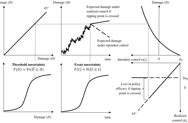
Crossing a tipping point may be unexpected for one of two reasons. Event uncertainty is a setting when a random event serves as the tipping point (lower middle subplot in Figure 1). This type of tipping point arises when irreversible environmental damage is caused by the duration of environmental degradation. For example, invasive species may unexpectedly become permanently established in a local area following a period of trade involving products known to harbor the invasive. If the random event occurs at some time 𝑡 = 𝑡̅, the uncertainty in the timing of the random event is captured by the cumulative distribution function 𝐹(𝑡) =

Pr(𝑡̅ ≤ 𝑡). In contrast, threshold uncertainty is a case where the system is described by a critical damage threshold 𝐷̅ beyond which restoration and healing are impossible (lower left subplot in

5_{For exposition, we assume the maximum damage is a hard boundary that may not be exceeded and treat 𝐷̿ as an}

(9)

9

Figure 1). Uncertainty in the location of the critical damage threshold is captured by the

cumulative distribution function 𝐹(𝐷) = Pr(𝐷̅ ≤ 𝐷). Under event uncertainty, the likelihood of reaching the tipping point is unaffected by the environmental degradation process 𝑑𝐷 since a tipping point is triggered by an exogenous random event. However, the environmental degradation process does increase the likelihood of crossing the tipping point under threshold uncertainty. Here shocks once small enough to avoid the tipping point (𝐷 < 𝐷̅) push the system over the tipping point 𝐷 ≥ 𝐷̅ rendering the control action ineffective.

The optimal policy implementation decision is depicted in Figure 2. A risk-neutral6 decision maker with a constant rate of time preference weighs the benefits and costs of delaying action by choosing at each instant in time: 1) the optimal stringency of the control strategy to be implemented (𝛼₁∗, 𝜎₁∗) and 2) whether a strategy with that level of stringency should be

implemented immediately or postponed until the next instant in time. We make two simplifying assumptions that allow a focus on the influence of irreversibility and uncertainty in certain contexts. First, the policy can be implemented only once. This places a significant weight on the opportunity cost of immediate action, as applicable to cases where political inflexibility or

institutional constraints make revisiting the policy unlikely. These types of institutional failures are common (Arrow et al. 2000) and particularly prevalent in issues surrounding tipping points (Horan et al. 2011)

Second, changes in system dynamics caused by crossing the tipping point are not

discernable to the decision maker prior to adopting the policy. If a decision maker continuously observes that a given level of damage did not exceed an unknown critical threshold, then the

6_{In the case of public investment, Arrow and Lind (1980) show that a risk neutral social planner may be justified if}

(10)

10

decision maker can be assured that all lower levels of damage are safe. In this case, the

instantaneous probability rate of crossing an unknown threshold is subject to a path dependency (Tsur and Zemel 1995, 1996). Increases in damage will only risk crossing the critical threshold if higher levels of damage have not already been experienced and deemed safe. Our assumption of an indiscernible tipping point may be more likely in natural systems where there is a lag between the variable of interest (i.e., damages) and the crossing of the tipping point. If crossing the tipping point is immediately discernable to the decision maker, Bayesian updating should be used to capture the path dependency that arises from learning about the tipping point (Groeneveld, Springborn and Costello 2014; Lemoine and Traeger 2014).

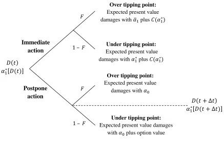
Since crossing the tipping point is not immediately discernable to the decision maker, immediate policy adoption and postponing policy adoption at any point in time is defined by lotteries where the payoff when above the tipping point occurs with probability F and the payoff when below the tipping point occurs with probability 1 - F. Immediate strategy implementation incurs C (with probability 1) but lowers 𝜎0 to 𝜎1∗ and 𝛼0 to 𝛼1∗ with probability (1 – F) or 𝛼̅1 with probability F. Otherwise the strategy is postponed until the next instant in time where the decision maker is faced with a similar lottery with payoffs and probabilities updated based on the new, realized value of D. In short, the decision maker chooses whether to implement the policy today based on the current lottery or postpone policy implementation and receive a new lottery. This dynamic lottery characterizes a wide range of environmental policy debates that center on the question of whether it is too late to act.

(11)

11

probabilities while the stringency decision influences the lottery payoffs. Implementing a control strategy becomes the preferred alternative when current damage reaches or exceeds a threshold D*. Implementing the strategy at this critical threshold will minimize the present value of expected damage and control cost into perpetuity. When current damage is below this

threshold it is optimal to delay the strategy until damage reaches or exceeds D*. If 𝐷(𝑡) reaches 𝐷∗_{before the tipping point, action will be optimally taken to avoid the irreversible damage} triggered by the tipping point. If 𝐷(𝑡) reaches 𝐷∗ after the tipping point, the best a decision maker can do is adopt a policy that would slow the transition to the inevitable level of damage 𝐷̿.

The relationship between the timing and stringency of the control strategy are shaped by the environmental and economic irreversibilities. The tipping point suggests that more stringent policies should be implemented early to avoid the likelihood of incurring large costs in exchange for a less effective policy. However, acting early increases the chance that damages will be lower than expected and previously incurred sunk costs will be viewed as excessive. To counter this possibility, a decision maker will either reduce the stringency of the early policy or delay the implementation of the more stringent policy (Buttle and Rondeau 2004). Whether the decision maker views policy expediency and stringency as complements or substitutes depends on which irreversibility is more influential.

3. Policy implementation as a choice between lotteries

(12)

12

point has been crossed, these payoffs are conditional on the tipping point having not yet been reached. Thus the payoff from immediate policy implementation and postponing

implementation at any point in time is defined by an implementation lottery 𝐿𝐼 and a continuation lottery 𝐿𝐶.

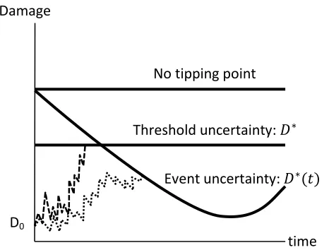
The inter-temporal policy decision described above critically depends on the nature of the tipping point uncertainty. When model variables are stochastic and the tipping point is unknown, one must distinguish between thresholds that delineate time (Zemel 2012) and thresholds that delineate regions of the state space (Brozović and Schlenker 2011).7 The former implies a tipping point is triggered by an exogenous random event and the likelihood of the system tipping increases with the passage of time (event uncertainty). The latter implies a tipping point is triggered by an unknown threshold in the state space and the likelihood of the system tipping increases in a system state variable (threshold uncertainty). Under event uncertainty the value of continuation and implementation lotteries changes over time causing the timing of mitigation to be defined by a threshold curve 𝐷∗(𝑡). In contrast, lotteries under threshold uncertainty do not change over time leading to a constant damage threshold that triggers policy adoption 𝐷∗.

3.1 Dynamic environmental lotteries under event uncertainty

Event uncertainty can be incorporated by assuming the threshold will be crossed at some unknown point in the future with likelihood determined by a hazard rate ℎ(𝑡) (Clarke and Reed

7_{If the model is deterministic, a critical state-space threshold can be translated to a critical point in time. Both cases}

(13)

13

1994; de Zeeuw and Zemel 2012; Tsur and Zemel 1998).8 Specifically, a conditional probability density function is defined over changes in time:

ℎ(𝑡) = lim

∆𝑡→0[Pr

(𝑡𝑖𝑝𝑝𝑖𝑛𝑔 𝑝𝑜𝑖𝑛𝑡 𝑏𝑒𝑡𝑤𝑒𝑒𝑛 𝑡 𝑎𝑛𝑑 (𝑡 + ∆𝑡)|𝑛𝑜 𝑡𝑖𝑝𝑝𝑖𝑛𝑔 𝑝𝑜𝑖𝑛𝑡 𝑢𝑛𝑡𝑖𝑙 𝑡)

∆𝑡 ] (2)

The conditional pdf or hazard function represents the instantaneous probability rate of crossing a tipping point at t given no irreversible environmental damage up until t. Ifℎ(𝑡)is constant the probability of crossing a tipping point is constant regardless of the current time, but if ℎ(𝑡)is increasing there will be a greater probability of crossing the tipping point the longer control is delayed. Equation (2) implies the probability of crossing a tipping point at time t is

𝐹(𝑡) = Pr(𝑡̅ ≤ 𝑡) = 1 − exp (− ∫ ℎ(𝜏)𝑡 0

𝑑𝜏) (3)

over support [0, ∞].9 The evolution of tipping risk under event uncertainty is governed by the differential equation 𝑑𝐹 𝑑𝑡⁄ = ℎ(𝑡)[1 − 𝐹(𝑡)] with 𝐹(0) = 0. Changes in tipping risk depend only on the hazard function and the decision maker knows that over some interval of time action can be taken that will reverse the accumulation of damage but eventually a tipping point will be crossed that makes damage irreversible.

The implementation lottery represents the discounted expected damage from immediate strategy implementation, and is a linear combination of the expected payoffs from immediate policy implementation when currently above (with probability F) and below (with probability 1 – F) the tipping point:

8_{Event uncertainty may arise in a number of ways. In some circumstances the threshold is known but one or more}

model variables are stochastic (e.g., Kolstad 1996; Saphores 2003). In other situations, model variables are deterministic and the threshold is unknown (e.g., Cropper 1976; de Zeeuw and Zemel 2012; Nævdal 2006).

9_{Allowing for the support of the distribution to include all non-negative values recognizes that the tipping point will}

(14)

14 𝐿𝐼_{(𝑡, 𝐷; 𝛼}

1, 𝜎1) = [1 − 𝐹(𝑡)]𝑊𝐼(𝐷; 𝛼1∗, 𝜎1∗) + 𝐹(𝑡)𝑊𝐼(𝐷; 𝛼̅1, 𝜎1∗) (4)

with 𝑊𝐼(𝐷, 𝛼₁∗, 𝜎₁∗) ≤ 𝑊𝐼(𝐷, 𝛼̅₁, 𝜎₁∗) since 𝛼₁∗ ≤ 𝛼̅₁. If the tipping point has been reached (with probability 𝐹(𝑡)), damages are irreversible and the decision maker receives the discounted expected damage with 𝛼̅1 = max[𝑏𝛼0, 𝛼1∗] from that point forward 𝑊𝐼(𝐷; 𝛼̅1, 𝜎1∗). If the tipping point has not been reached, the decision maker receives 𝑊𝐼(𝐷; 𝛼₁∗, 𝜎₁∗). The cost associated with holding this lottery will increase as damages increase (𝜕𝐿𝐼⁄𝜕𝐷> 0) since discounted expected damages must increase in the current level of damage (𝜕𝑊𝐼⁄𝜕𝐷> 0).

Given current damages 𝐷(𝑡), the optimal degree of policy stringency (𝛼₁∗, 𝜎₁∗) is found by minimizing the expected damages and policy costs from that point forward:

min 𝛼1,𝜎1{𝐿

𝐼_{(𝑡, 𝐷; 𝛼}

1, 𝜎1) + 𝐶(𝐷; 𝛼1, 𝜎1)} (5)

For 𝛼₁∗ ≥ 𝑏𝛼0, the optimal stringency is not constrained when the tipping point has been reached. Here, the timing of policy implementation is not directly affected by the tipping point and can be solved for using well-known stochastic dynamic programming methods (Dixit and Pindyck 1994). For 𝛼₁∗ ≥ 𝑏𝛼₀, the timing of policy implementation is influenced by the presence of the tipping point.

The continuation lottery represents the expected payoff from postponing strategy implementation, and is a linear combination of the expected payoffs from postponing policy implementation when currently above (with probability 𝐹(𝑡)) and below (with probability 1 − 𝐹(𝑡)) the tipping point:

(15)

15

with 𝑊𝐶 < 𝜑 for all t. The policy implementation opportunity can be optimally deployed (optimal level of stringency implemented when 𝐷 = 𝐷∗) if the tipping point has not been reached (with probability 1 − 𝐹(𝑡)). In this case, the decision maker receives the value of the option to delay implementation, 𝑊𝐶, which is composed of the discounted expected damage from doing nothing, 𝜑(𝐷), and the option value Ω(𝑡, 𝐷). The option value reflects the economic value of being able to update the policy strategy in response to new information on the level of environmental damage. Due to economic irreversibility, this ability to update is lost once the strategy is implemented. Thus, the option value is often referred to as the value of information conditioned on inaction. Here the option value is also conditioned on not yet crossing the tipping point since crossing the tipping point also eliminates the ability to update by constraining policy options. Because damage is modeled as a positive value, this option value is a nonpositive cost of immediate action as it has a damage reducing character. If the tipping point has been reached (with probability 𝐹(𝑡)), the policy implementation opportunity cannot be optimally deployed (the policy option has expired as stringency is now limited to 𝛼̅₁) and the option value goes to zero. Here, the payoff from delay is the expected net present value of damage from doing nothing, 𝜑(𝐷) with 𝜕𝜑 𝜕𝐷⁄ > 0.

(16)

16

𝜌𝐿𝐶 _{= 𝐷(𝑡) +}𝐸[𝑑𝐿𝐶]

𝑑𝑡 (7)

where 𝜌 is the risk-free discount rate (see supplemental appendix for derivation). In financial terms, the decision maker faces an obligation to the flow of environmental damages. The obligation is treated as an asset whose value 𝐿𝐶 must be optimally managed (i.e., minimized). Since the most stringent policy options become unavailable, crossing the tipping point

effectively serves as an unexpected expiration date on the option associated with mitigating this environmental damage. The Bellman equation acts as an equilibrium condition ensuring a willingness to postpone the policy over the time interval dt prior to strategy implementation. Since 𝐿𝐶 is a function of D, we can apply Ito’s Lemma to find 𝐸[𝑑𝐿𝐶]/𝑑𝑡 and substitute into (7) to find:

𝜌𝐿𝐶 _{= 𝐷(𝑡) +}𝜕𝐿𝐶

𝜕𝑡 + 𝛼0(𝐷) 𝜕𝐿𝐶

𝜕𝐷 + 1

2𝜎02(𝐷) 𝜕2_𝐿𝐶

𝜕𝐷2 (8)

Using (6) we can rewrite in terms of the unknown value function 𝑊𝐶(𝑡, 𝐷)

𝜌𝑊𝐶 _{= 𝐷 +}𝐸[𝑑𝑊𝐶]

𝑑𝑡 [1 − 𝐹]+ 𝐸[𝑑𝜑]

𝑑𝑡 𝐹 +[𝜌𝐹 − 𝐹̇ ][𝑊

𝐶_{− 𝜑}_]₍₉₎

where 𝐹̇ is the time derivative of tipping point risk and

𝐸[𝑑𝑊𝐶_]

𝑑𝑡 =

𝜕𝑊𝐶

𝜕𝑡 + 𝛼0(𝐷) 𝜕𝑊𝐶

𝜕𝐷 + 1

2𝜎02(𝐷) 𝜕2_𝑊𝐶

𝜕𝐷2 , (9𝑎)

𝐸[𝑑𝜑]

𝑑𝑡 = 𝛼0(𝐷) 𝜕𝜑 𝜕𝐷+

1

2𝜎02(𝐷) 𝜕2_𝜑

(17)

17

The differential equation in (9) holds for all values in the continuation region of the state-time space (namely 𝐷(𝑡) < 𝐷∗(𝑡)) and is used to solve for the continuation value function 𝑊𝐶.10 The left-hand side is the return a decision maker would require to delay policy implementation over the time interval dt. The right-hand side is the expected return from delaying policy

implementation over the interval dt. Specifically, delaying strategy implementation results in current damages D plus the expected capital losses in this context of damage minimization.

The complete description of a policymaker’s response (𝐷∗_{(𝑡), 𝛼}

1∗(𝑡), 𝜎1∗(𝑡)) is found by solving the differential equation in (9) and simultaneously solving the optimality conditions associated with (5) evaluated at 𝐷∗(𝑡), an initial condition 𝑊𝐶(0, 𝐷), and a pair of boundary conditions (Dixit 1991): 𝐿𝐶(𝑡, 𝐷∗) = 𝐿𝐼(𝐷∗; 𝛼₁∗, 𝜎₁∗) + 𝐶(𝐷∗; 𝛼₁∗, 𝜎₁∗) and 𝐿𝐶_𝐷(𝑡, 𝐷∗) =

𝐿𝐼𝐷(𝐷∗; 𝛼1∗, 𝜎1∗).11 The initial condition ensures the continuation value function equals the relevant value function when there is no risk of crossing a tipping point: 𝐹(0) = 0. The first boundary condition requires the lottery received from postponing policy adoption equal the lottery from immediate policy adoption at (𝐷∗(𝑡), 𝛼₁∗(𝑡), 𝜎₁∗(𝑡)). The second boundary requires the continuation and implementation lotteries meet tangentially at 𝐷∗(𝑡) so that expected payoffs are also balanced at the margin. These boundary conditions are the familiar value matching and smooth pasting conditions written in terms of the lotteries that arise with the addition of tipping point uncertainty. Unfortunately an analytic solution is intractable when a tipping point exists. However, a general characterization of the optimal policy response is presented in Figure 3.

10_{Provided closed-form expressions for}_F_{and 𝜑, equation (9) is a second-order linear partial differential equation}

(PDE) with nonconstant coefficients. Because the only second derivative is with respect to D, this is a parabolic PDE similar to the heat equation.

11

(18)

18

Initially, 𝐹(0) = 0 and the Bellman equation collapses to the form familiar in the traditional real options literature where a tipping point is absent. As time passes, the capital losses are probabilistic (second and third terms) and must capture how the probability of exceeding the tipping point changes with respect to time (fourth term). The second and third terms unambiguously increase the expected damages from delaying policy implementation. The probability the tipping point may have already been exceeded or will be exceeded if time passes encourages more immediate action.

However, the sign of the fourth term is ambiguous and depends on a golden rule condition for mitigation investments in the face of tipping point risk. This term captures an additional effect of the option value, [𝑊𝑐 − 𝜑] < 0, which arises in the opposing irreversibility setting. Initially, the probability of the random event rises faster than the discount rate, 𝐹̇ 𝐹⁄ > 𝜌. During this period of time the expected damage from holding the continuation lottery increases proportionally to the option value which hastens policy implementation. Since your policy option may expire at the next instant in time, the random event works to hasten policy implementation and the larger the option value the greater the incentive to act quickly.

(19)

19

in the absence of a random event that triggers irreversible damage. If the fourth term on the right hand side of (9) dominates all other terms, it is possible that the random event delays policy

implementation beyond the decision threshold suggested in the absence of a tipping point.

3.2 Dynamic environmental lotteries under threshold uncertainty

Many tipping points are triggered when a state variable crosses a critical threshold (Nævdal 2006; Tsur and Zemel 1996). This makes the use of a traditional hazard function problematic since the passage of time does not necessarily mean an increase in damage and a more impending tipping point. We adopt a combined approach where 𝐷̅ is a real-valued random variable and the uncertainty in 𝐷̅ is controlled with distribution function 𝐹(𝐷) = Pr(𝐷̅ ≤ 𝐷) and density function 𝑑𝐹 𝑑𝐷⁄ over support [0, ∞].12 Since the tipping point is defined as a critical level of damage, a conditional probability density function is defined over changes in damage instead of changes in time:13

ℎ(𝐷) = lim

∆𝐷→0[Pr

(𝑡𝑖𝑝𝑝𝑖𝑛𝑔 𝑝𝑜𝑖𝑛𝑡 𝑏𝑒𝑡𝑤𝑒𝑒𝑛 𝐷 𝑎𝑛𝑑 (𝐷 + ∆𝐷)|𝑛𝑜 𝑡𝑖𝑝𝑝𝑖𝑛𝑔 𝑝𝑜𝑖𝑛𝑡 𝑢𝑛𝑡𝑖𝑙 𝐷)

∆𝐷 ] (10)

with 𝑑ℎ 𝑑𝐷⁄ > 0 reflecting a greater probability of irreversible damage the more the system is disturbed. The conditional pdf or hazard function represents the instantaneous probability rate of reaching a tipping point at D given no irreversible environmental damage up until D. Equation (10) implies the probability a level of damage D has reached the tipping point is

𝐹(𝐷) = Pr(𝐷̅ ≤ 𝐷) = 1 − exp (− ∫ ℎ(𝑠) 𝐷 0

𝑑𝑠) (11)

12_{Allowing for the support of the distribution to include all non-negative values recognizes that a tipping point may}

not exist.

13_{The conditional pdf is related to the density function through ℎ(𝐷) =}𝑑𝐹 𝑑𝐷⁄

1−𝐹 . The specification is similar in spirit

(20)

20

Unlike event uncertainty, the evolution of tipping risk under threshold uncertainty is determined by both the distribution function 𝐹 and the stochastic damage process. Since 𝐹 is a function of

D, we can apply Ito’s Lemma to find

𝑑𝐹 = [𝛼0(𝐷) 𝜕𝐹 𝜕𝐷+

1

2𝜎02(𝐷) 𝜕2_𝐹

𝜕𝐷2] 𝑑𝑡 + 𝜎0(𝐷) 𝜕𝐹

𝜕𝐷𝑑𝑧 (12)

subject to a pair of reflecting barriers at 𝐹 = 0 and 𝐹 = 1 that ensure 0 ≤ 𝐹 ≤ 1. Equation (12) implies F is a stochastic variable with its own expected value and variance.14 Specifically, the probability of reaching the tipping point stochastically evolves as damage stochastically moves up the cumulative distribution function. Stochastic tipping risk reflects the compound

distribution of F and D that arises from the combination of threshold uncertainty and uncertainty in system dynamics.15

The problem under threshold uncertainty is similar to the problem under event

uncertainty except 1) lottery probabilities are a function of damage instead of time and 2) the option value and continuation value function do not depend on calendar time t. In other words, since the probability of losing the policy option does not depend on time, the option value is only influenced by the evolution of D and not the passage of time.16 This changes the partial

14_{A reflecting barrier means that if}_F_{= 0 (}_F_{= 1) and the next increment}_dF_{is negative (positive), then the sign of}

the increment is reversed. Essentially, the stochastic process for F is allowed to proceed according to the stochastic differential equation so long as 0 < F < 1.

15_{If the threshold were unknown but future damages were known with certainty (𝜎}

0= 0), the future probability of

crossing the tipping point would increase at 𝛼0(𝐷)𝜕𝐹_𝜕𝐷 but would be known with certainty in the future. Likewise,

with stochastic damages and 𝐷̅ known withcertainty, the probability of crossing the tipping point is characterized by a known distribution at all points in time Ψ(𝑡) = Pr(𝐷̅ ≤ 𝐷|𝐷0) = 1 − ∫ 𝜓(𝐷₀𝐷̅ 0, 𝑡0; 𝑢, 𝑡)𝑑𝑢 where

𝜓(𝐷0, 𝑡0; 𝐷, 𝑡) is the density function for the generalized Ito damage process with 𝐷0 the initial value at time 𝑡0.

The density function is known and is the solution to a Kolmogorov forward equation (Karlin and Taylor 1981).

16_{Mathematically, the model with event uncertainty is a finite horizon optimal stopping problem while the model}

(21)

21

differential equation in (9) to the following ordinary differential equation (see supplemental appendix for derivation)

𝜌𝑊𝐶_{= 𝐷 +}𝐸[𝑑𝑊𝐶]

𝑑𝑡 [1 − 𝐹] +

𝐸[𝑑𝜑]

𝑑𝑡 𝐹 + [𝜌𝐹 −

𝐸[𝑑𝐹]

𝑑𝑡 ] [𝑊𝑐− 𝜑] + 𝜎02(𝐷) 𝜕𝐹 𝜕𝐷[

𝜕𝜑 𝜕𝐷−

𝜕𝑊𝐶

𝜕𝐷 ] (13)

where

𝐸[𝑑𝑊𝐶_]

𝑑𝑡 = 𝛼0(𝐷) 𝜕𝑊𝐶

𝜕𝐷 + 1

2𝜎02(𝐷) 𝜕2_𝑊𝐶

𝜕𝐷2 , (13𝑎)

𝐸[𝑑𝐹]

𝑑𝑡 = 𝛼0(𝐷) 𝜕𝐹 𝜕𝐷+

1

2𝜎02(𝐷) 𝜕2_𝐹

𝜕𝐷2 (13𝑏)

and 𝐸[𝑑𝜑]/𝑑𝑡 defined by (9b). The complete description of a policymaker’s response (𝐷∗_{, 𝛼}

1∗, 𝜎1∗) is found by solving the differential equation in (13) and simultaneously solving similar versions of the optimality conditions for 𝛼₁∗ and 𝜎₁∗ and boundary conditions. An analytic solution remains intractable but general insights are possible (see Figure 3).

There are three key differences in the optimal timing of a policy response between event uncertainty and threshold uncertainty. First, as equation (13) is an ODE instead of the PDE in equation (9), policy implementation is triggered by crossing a constant critical damage threshold 𝐷∗_{instead of the threshold curve}_𝐷∗_(𝑡)_{as found with event uncertaity. When current damage is} below this threshold it is optimal to delay action until damage reaches or exceeds D*. If 𝐷∗ < 𝐷̅, action will be taken before reaching the tipping point. If 𝐷∗ ≥ 𝐷̅, the best a decision maker can do is delay the inevitable 𝐷̿. The likelihood of the latter is given by 𝐹(𝐷∗).

(22)

22

term unambiguously increases the expected damages from delaying policy implementation. While the passage of time will not necessarily imply a more impending irreversible threshold, an increase in damage does increase the risk of irreversible damage.

Third, the golden rule condition for tipping risk now depends on the expected change in the risk of tipping: 𝐸[𝑑𝐹]_𝑑𝑡 . Specifically, an uncertain tipping point threshold hastens policy implementation if 𝐸[𝐹̇] 𝐹⁄ > 𝜌 and delays policy implementation if 𝐸[𝐹̇] 𝐹⁄ < 𝜌. Under event uncertainty, this golden rule condition is a function of the decision maker’s discount rate and the hazard function. From (13b), the golden rule condition under threshold uncertainty is also influenced by the environmental degradation process 𝑑𝐷. This provides another channel for the uncertainty in future environmental damage to influence timing.

(23)

23

stationary policy target (risk reduction decisions based on 𝐷∗ instead of 𝐷∗(𝑡)), it will not necessarily result in more expedient policy action.

General insight about the relationship between uncertainty and timing of policy response are elusive in the context of an unknown threshold. Increases in stochasticity, 𝜎0, will work to delay policy implementation by decreasing the second and third terms. But more stochasticity will also hasten policy implementation by increasing the fifth term. The effect of stochasticity on the fourth term depends on the current level of damage.17 The effect of tipping point uncertainty is slightly less ambiguous. When damage is small, tipping point uncertainty unambiguously expedites implementation. As damage increases, the effect of tipping point uncertainty becomes ambiguous.

4. Illustrative example: Asian carp invasion into the Great Lakes

To illustrate the usefulness of the model, we apply it to the spread of invasive Asian carp. Asian carp were initially introduced into the Mississippi River and have gradually been

spreading north causing vast amounts of damage to fisheries and impacts to biodiversity

(Garvey, Ickes and Zigler 2010). The Mississippi River is linked to the Great Lakes through the Illinois waterway (Illinois River, Des Plaines River, Chicago Ship and Sanitary Canal).

Conventional wisdom indicates that the spread of Asian carp into the Great Lakes is an

irreversible event – once they establish in Lake Michigan it will be impossible to eradicate them

17

When 𝜕2𝐹

𝜕𝐷2> 0, more stochasticity increases 𝐸[𝐹̇] and, in turn, increases expected damages from delay. When

𝜕2_𝐹

(24)

24

from the Great Lakes. However, it’s unclear how far or how long carp must spread before they become established in Lake Michigan making this an unknown tipping point. Further, future spread of Asian carp is unknown due to environmental shocks and imperfect monitoring and detection. For instance, the electrofishing method used to capture/detect Asian carp may not be capturing the first individual to enter the system (Jerde et al. 2014), which compromises the ability to accurately predict the evolution of the invasion.

4.1 Characterizing the invasion and policy options

Bighead and Silver carp were discovered in the Illinois waterway in 1986 and 1998 respectively and have a known range extending into the Chicago Ship and Sanitary Canal (nearly 300 river miles). We assume future spread of Asian carp in the Illinois waterway is uncertain. Research indicates that the invasion front for both Bighead and Silver carp advances linearly (Jerde et al. 2014) suggesting that the number of Illinois Waterway river miles invaded (x) may be modeled with the following stochastic differential equation

𝑑𝑥 = 𝑟₀𝑑𝑡 + 𝑠₀𝑑𝑧 (14)

where 𝑟₀ is the current spread rate, 𝑠₀ is the current standard deviation of the spread process, and

dz is the increment of a standard Wiener process. The drift and volatility parameters are

(25)

25

Pecuniary damage from Asian carp is an exponential function of the river miles invaded 𝐷(𝑡) = 𝐷₀𝑒𝛾𝑥(𝑡)_where_𝐷

0 is the amount of damage when carp initially invaded the Illinois Waterway (when x = 0) and 𝛾 is a positive parameter. Since damage is a function of x, its current evolution is described by the geometric Brownian motion (GBM) 𝑑𝐷 = 𝛼₀𝐷𝑑𝑡 + 𝜎₀𝐷𝑑𝑧 where 𝛼₀ = 𝑟₀𝛾 + (𝑠𝛾)2⁄2 and 𝜎₀ = 𝑠₀𝛾. The generality of GBM is attractive but it also has two particularly desirable properties for many environmental applications. First, by not reaching 0 in any finite time, GBM rules out negative levels of damage. Second it allows damage to accelerate which is often the result of increased human influence as damages grow. However, it assumes damage is unbounded which is inconsistent with the implications of an Asian carp invasion. We capture an upper bound on damage by assuming 𝐷̿ is an absorbing barrier. This limits the upside potential for damage making the damage process log-normally distributed over the range [0, 𝐷̿] only. Since damage follows a bounded GBM process the expected discounted damages from never intervening in the invasion process is

𝜑 = 𝐷(𝑡) (𝜌 − 𝛼0)−

𝛼₀𝐷̿

𝜌(𝜌 − 𝛼₀)𝐷̿𝜀0𝐷(𝑡)

𝜀0 (15)

with 𝜀₀ = (1₂−_𝜎𝛼0

02) + √(

𝛼0

𝜎02−

1 2)

2 +_𝜎2𝜌

02 > 0.

18

Due to a lack of data to guide our choice of damage function parameters, we assume 𝛾 = 0.005 and 𝐷₀ = 3 which implies damages are accumulating at 10% annually with a 13% deviation around this trend (𝛼₀ = 0.10; 𝜎₀ = 0.13) and carp must spread 700 miles (twice the length of Lake Michigan) to cause $100 million in damages. To estimate the maximum level of

18_{The upper barrier ensures expected damages are finite which precludes the traditional assumption 𝜌 > 𝛼} 0 and

(26)

26

annual damages associated with a complete invasion of the Great Lakes we adapt the findings of McIntosh et al. (2010), who estimate how much households would be willing to pay to delay aquatic invasions. As a lower bound, consider the willingness to pay of households in the two major cities on Lake Michigan, Chicago (1,194,337 in the 2010 U.S. Census) and Milwaukee (232,188 in the 2010 U.S. Census). McIntosh et al. found households are willing to make a one-time payment of $48 to delay low to high impacts one year. For households in these two cities, the aggregate willingness to pay is $68.5 million. Since these two cities constitute approximately 70% of the population that lives along Lake Michigan, we assume 𝐷̿ = 100 million.19 Figure 4B shows 𝐷 based on carp spread data, the expected path for damage, and Monte Carlo simulations of the bounded GBM damage process.

There are a number of potential policy options which have been implemented or are being considered to stop Asian carp from reaching the Great Lakes. For example, an electric barrier was built in the Chicago Ship and Sanitary Canal in 2002. Another proposal that has generated considerable debate is to close the Chicago Ship and Sanitary Canal to boat and barge traffic. Both of these policy options are aimed at reducing the rate of invasion but also introduce economic irreversibility due to their significant sunk costs. We assume a policy that has no effect on the volatility of damages and set 𝑐_𝛼= 50,000 such that the marginal cost of damage trend reduction is $100,000. This also implies the cost of stopping damage accumulation is $500 million which is consistent with annual economic impact estimates of shipping lock closure that range from $70 million to $190 million (Egan 2010). We also assume 𝑏 = 0.75, which suggests that crossing the tipping point significantly limits available policy options but does not render a policy completely ineffective. If the tipping point has been reached, the decision maker receives

(27)

27 𝑊𝐼_{(𝐷, 𝛼̅}

1) = 𝐸𝑡∫ 𝐷(𝜏)𝑒−𝜌(𝜏−𝑡)𝑑𝜏 ∞

𝑡

= 𝐷(𝑡) (𝜌 − 𝛼̅1)−

𝛼̅1𝐷̿

𝜌(𝜌 − 𝛼̅₁)𝐷̿𝜀̅1𝐷(𝑡)

𝜀̅1 (16)

with 𝜀̅₁ = (1₂−_𝜎𝛼̅₂1) + √(_𝜎𝛼̅1₂−1₂) 2

+2𝜌_𝜎₂ > 0. If the tipping point has not been reached, the

decision maker receives

𝑊𝐼_{(𝐷, 𝛼} 1∗) =

𝐷(𝑡) (𝜌 − 𝛼₁∗₎−

𝛼₁∗_𝐷_̿

𝜌(𝜌 − 𝛼₁∗_)𝐷̿𝜀1∗𝐷(𝑡)

𝜀1∗ (17)

with 𝜀₁∗ = (1₂−𝛼1

∗

𝜎2) + √(

𝛼₁∗

𝜎2−

1 2)

2

+2𝜌_𝜎₂ ≥ 𝜀̅1. Together, equations (15) – (17) capture how the expected payoffs of the policy lottery are influenced by a “control the spread” policy, the tipping point that signifies Asian carp establishment in the Great Lakes, and the transition to a new equilibrium level of damage 𝐷̿.20

4.2 Policy response to an invasion tipping point

While it is generally agreed that Asian carp establishment in the Great Lakes cannot be reversed, it is less clear whether this tipping point should be viewed as the crossing of a critical invasion threshold or a random event. The probability of establishment depends on 1) the frequency of invasive introduction events and 2) the number of invasive individuals introduced in a single introduction event (Leung, Drake and Lodge 2004; Lockwood, Cassey and Blackburn 2005). An invasive population front advancing closer to Lake Michigan likely increases the

20_{The first term in 𝑊}𝐼_{and 𝜑 is discounted expected damage when ignoring the alternative equilibrium 𝐷̿. The}

(28)

28

probability of establishment along both of these dimensions and lends support to the threshold concept. However other sources of human-mediated introduction (fish stocking, movement of live bait, intermittent hydrological connections) may also result in establishment independent of the location of the invasion front in the Chicago Ship and Sanitary Canal. These

human-mediated introductions suggest a random event may be more likely to trigger a tipping point. We consider both possibilities to highlight how divergent policy recommendations may originate from different perspectives of the invasion tipping point.

If risk of Asian carp establishment in the Great Lakes is thought to be primarily

determined by human-mediated introduction, the risk of establishment is dependent only on the passage of time. In this case, the unknown invasion tipping point is described by event

uncertainty with hazard function ℎ(𝑡). The specification of the hazard function critically depends on whether the hazard is unimodal or monotone. A flexible parametric form that accommodates both is the Weibull model with ℎ(𝑡)= 𝜆𝑡𝛽−1 where 𝜆 > 0 and β is a shape parameter with a value greater than one.21 Applying this specification to (3) we find

𝐹(𝑡) = 1 − exp (−𝜆𝑡 𝛽

𝛽 ) (18)

With few measures of the risk of Asian carp establishment in the Great Lakes, we assume 𝛽 = 2 and 𝜆 = 0.019. These values imply that there was a 75% probability that a random event occurred that triggered irreversible establishment in the Great Lakes in 2009. Figure 4C shows 𝐹(𝑡) under event uncertainty.

21_{The mean and variance of a Weibull random variable are 𝐸[𝑡̅] = (}𝛽

𝜆)

1

𝛽_{Γ (1 +}1

𝛽) and var[𝑡̅] = ( 𝛽

𝜆)

1

𝛽_{[Γ (1 +}2

𝛽) −

(Γ (1 +1_𝛽))

2

(29)

29

Alternatively, if risk of Asian carp establishment in the Great Lakes is dependent only on the gradual expansion of invaded area in the Illinois River, the invasion tipping point is described by threshold uncertainty with hazard function ℎ(𝐷). For consistency we assume the Weibull model also characterizes threshold uncertainty: ℎ(𝐷) = 𝜆𝐷𝛽−1 and 𝐹(𝐷) = 1 − exp (−𝜆𝐷

𝛽

𝛽 ). We also assume 𝛽 = 2 and 𝜆 = 0.019 which implies a 79% probability that the 2009 invasion front had crossed a critical threshold that triggered irreversible establishment in the Great Lakes. Figure 4C shows 𝐹(𝑡) under threshold uncertainty based on carp spread data, the expected path for 𝐹(𝑡), and Monte Carlo simulations of the stochastic 𝐹(𝑡) process.

(30)

30

invasion with the risk of irreversibly crossing a tipping point. Additional delays in policy adoption increase the probability that carp have established in Lake Michigan, makes it more likely that any policy will only lower the damage accumulation rate to 𝑏𝛼₀ = 0.075, and reduces incentives for any policy more stringent than this level.22

We also consider the optimal timing of a policy 𝐷𝑠𝑡𝑜𝑝 that would stop the accumulation of damages 𝛼₁ = 0. While clearly a second-best deviation from 𝛼₁∗ = 0.041, considering a more stringent policy is insightful for a number of reasons. First, political pressure may force decision makers to forgo policies that slow spread and focus exclusively on policies that would stop any additional damage. Second, stopping the accumulation of damage (instead of slowing the spread) may also be more consistent with the proposed hydro-separation of the Mississippi and Great Lakes watersheds currently being considered. Third, policy makers are often limited to a few policy options precluding the ability to select from a continuum of policy stringencies. Finally, and perhaps more generally, a policy with 𝛼₁ = 0 may reflect a strong interpretation of the precautionary principle which supports preventative actions in the face of possible

irreversible harm to the environment (Gollier, Moldovanu and Ellingsen 2001). Because of its larger cost, there is an incentive to adopt this policy earlier 𝐷𝑠𝑡𝑜𝑝 < 𝐷∗ since the losses from crossing a tipping point (lost sunk costs) are larger. On the other hand, its larger cost also makes policy makers more wary of committing these large costs to an environmental problem that may not be as damaging as previously thought, 𝐷𝑠𝑡𝑜𝑝 > 𝐷∗.

22_{For example, the most recent 2009 estimate of the invasion front implies damages have grown to approximately}

𝐷2009= $12.8 million. A more damaging invasion suggests a more stringent policy. However, the probability that

(31)

31

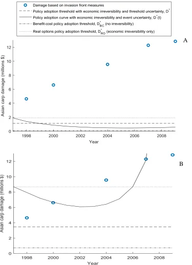
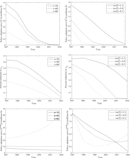
In our illustrative example, deviating from the optimal but less stringent policy to this precautionary policy will lead to a less expedient response for both types of tipping point (Figure 5B). Under threshold uncertainty, the precautionary policy should only be adopted when

damage reaches 𝐷𝑠𝑡𝑜𝑝 = $3.4 million. Since 𝐷0 = $3 million, adopting the more precautionary policy could have been justified shortly after Asian carp entered the Illinois waterway in 1997 and would continue to be justified thereafter. Under event uncertainty, the damage does not reach the critical threshold curve 𝐷𝑠𝑡𝑜𝑝(𝑡) until 2000. But since the passage of time increases the likelihood that Asian carp have already established in Lake Michigan, adoption of the more stringent policy becomes more risky and as a result more difficult to justify in the future. Without the ability to choose a less stringent policy in the face of this increasing risk, decision makers find it optimal to delay this more precautionary policy further into the future. By 2009, a precautionary policy that would have been optimal in previous years becomes too risky to justify the sunk costs: 𝐷𝑠𝑡𝑜𝑝(2009) > 𝐷₂₀₀₉. When options are limited to the most stringent policies and action must be taken before it’s too late, a tipping point forces policy adoption to take place within a window or interval of time.

4.3 The relative influence of opposing irreversibilities

(32)

32

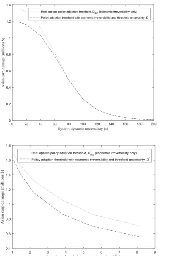
point irreversibility. The second uses a traditional real options methodology to identify a critical damage threshold 𝐷_𝑅𝑂∗ that considers the policy’s option value (economic irreversibility) but does not consider the tipping point (see supplemental appendix for derivation). For consistency, each rule is evaluated for a policy that would reduce the rate of damage accumulation to 𝛼₁∗. By comparing these critical thresholds to 𝐷∗ and 𝐷∗(𝑡), we can identify the influence of each irreversibility on the timing of the policy decision.

Figure 5A shows the four critical policy adoption thresholds. As expected, the inclusion of economic irreversibility and the associated option value suggests policy adoption should be delayed longer than suggested under traditional benefit-cost analysis: 𝐷_𝑅𝑂∗ > 𝐷_𝐵𝐶∗ . The inclusion of the tipping point works to reduce the option value and hasten policy adoption. However, 𝐷∗ and 𝐷∗(𝑡) do not fall below 𝐷_𝐵𝐶∗ suggesting that an unknown tipping point, regardless of whether it is triggered by crossing a threshold or a random event, reduces but does not eliminate the influence of the option value that arises due to the presence of sunk costs. In other words, an option to mitigate environmental damage is still valuable even if that option may unexpectedly expire once a tipping point is crossed.

4.4 The precaution-uncertainty relationship with opposing irreversibilities

(33)

33

variance of 𝐷̅.23 Changes in 𝐷𝑠𝑡𝑜𝑝 reflect the impact of uncertainty on the timing of mitigation only whereas changes in 𝐷∗ reflect the combined effect on timing and stringency.

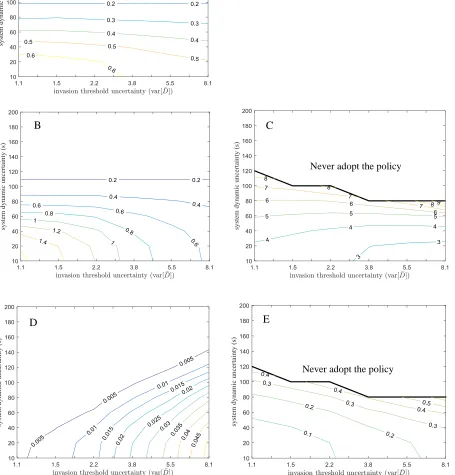
For the precautionary policy (𝛼₁ = 0), less knowledge about system dynamics leads to an expected delay in policy adoption (larger 𝐷𝑠𝑡𝑜𝑝) and a greater likelihood the tipping point will have been reached by the time the policy is adopted. The delay is due to increases in the policy’s option value which captures the decision maker’s hesitance to commit sunk costs to control an invasion which is more uncertain. The effect of increases in threshold uncertainty depends on how well the system dynamics are understood. When stochasticity is low, increases in threshold uncertainty lead to more immediate policy adoption. But when stochasticity is high, additional threshold uncertainty leads to an expected delay in policy adoption. Both types of uncertainty may be so large that the expected return from investing in a policy that stops the accumulation of damage will always be less than the decision maker’s required return 𝜌 indicating that the policy should never be adopted.

When policy makers are free to choose the stringency of the policy, uncertainty has drastically different effects on the policy decision. Increases in both types of uncertainty lead to more immediate policy adoption but a less stringent policy. Even though the policy is being adopted sooner, increases in threshold uncertainty make it more likely the tipping point has been reached when the policy is implemented. At very high levels of stochasticity, threshold

uncertainty does not influence the policy decision. When 𝑠 increases to 100, the optimal policy is so immediate that it must be paired with a lax policy 𝛼₁∗ > 𝑏𝛼₀, eliminating any consequences from reaching the tipping point and any incentive to avoid it. Thus, the commonly held belief

23_{Evaluating the effect of uncertainty through changes in the mean-preserving spread rules out outcomes that will be}

(34)

34

that more uncertainty leads to a delay in the commitment of sunk costs only arises when there is an inability to choose the amount invested.

To understand these disparate results, note that threshold uncertainty affects the

probability of reaching the tipping point in the current period and expectations of reaching it in the future. Impacts on the current probability affect the stringency decision through increases in

F which lowers the marginal benefit of a more stringent policy. From equation (12), more threshold uncertainty also affects expectations of reaching the tipping point in the future. If 𝜕2_{𝐹 𝜕𝐷}_⁄ 2_{increases as a result of more threshold uncertainty, expectations of avoiding the} tipping point look worse in the short run creating an incentive to hasten the policy response. If increased threshold uncertainty decreases 𝜕2𝐹 𝜕𝐷⁄ 2, expectations for avoiding the tipping point look better in the short run creating an incentive to delay the policy response.24 These second-order effects will be minor when stochasticity is low.

In contrast, stochasticity is a dynamic form of uncertainty that only affects expectations of reaching the tipping point in the future. This type of uncertainty affects the timing of the policy response in two ways. The first is through increases in the option value, which trigger a delayed response. At the low damage thresholds seen in Figure 6, more uncertainty in system dynamics causes a decision maker to be more pessimistic about crossing the tipping point threshold in the immediate future. The increase in stochasticity thus creates an opposing incentive for policy makers to hasten their policy response to preempt the unknown threshold.

While the impact of event uncertainty is qualitatively similar to results with threshold uncertainty (Figure 7), the impact of uncertainty depends on how much time has passed. When

24_{Note that the impact of changes in 𝜕𝐹 𝜕𝐷}_⁄ _{on the optimal timing of mitigation is netted out. Essentially, one is}

(35)

35

decision makers are limited to the precautionary policy that stops damage when 𝐷(𝑡) = 𝐷𝑠𝑡𝑜𝑝_(𝑡)_{, more uncertainty in the timing of the random event hastens policy adoption prior to} 2001 but delays policy adoption thereafter (bottom right panel in Figure 7). Thus it is not clear whether more information about the timing of a random event that triggers a tipping point will hasten or delay efforts to prevent further damage.

4.5 Differing perceptions of irreversibility

An alternative interpretation of 𝐷_𝑅𝑂∗ is the critical policy adoption threshold employed by individuals who do not believe that a tipping point is irreversible. The difference between 𝐷_𝑅𝑂∗ and 𝐷∗ (or 𝐷∗(𝑡)) then reflects disagreements over policy implementation between groups who have different beliefs over the ability of the natural system to recover. Since there is often little precedent for tipping points, different perceptions of the implications of crossing a tipping point are likely common. From Figure 5, these disagreements will be more pronounced when focusing exclusively on precautionary policies. More common ground will likely be found by focusing on less stringent policies. It is also interesting to note that 𝐷𝑠𝑡𝑜𝑝(𝑡) > 𝐷_𝑅𝑂𝑠𝑡𝑜𝑝 after 2006. Individuals who believe a tipping point will be triggered by a random event will eventually become more pessimistic about returns from the mitigation investment and will advocate for delaying mitigation longer than their counterparts who do not believe a tipping point exists.

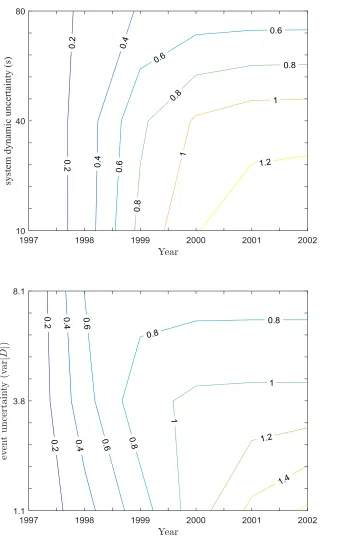
Figure 8 shows that these disagreements may be partially alleviated by reducing

uncertainty in the location of the unknown threshold. Lowering this source of uncertainty places less emphasis on the irreversibility associated with crossing a tipping point. Surprisingly

(36)

36

invasion process. Eventually decreasing either type of uncertainty leads to greater disagreement between those that view tipping points as irreversible and those that do not.

5. Conclusions

Environmental tipping points create three specific incentives to act sooner rather than later. First, expected damages from delay are probabilistic and are larger than they would be without the tipping point. Second, the expected benefits from policy implementation are reduced due to the possibility the policy will not be as effective as expected if the tipping point has been crossed. This creates an incentive for less stringent and less costly policies that will be easier to justify at lower levels of environmental damage which indirectly works to speed up a policy response. Third, the possibility that delay might cause the system to tip introduces the possibility that the option to avoid the tipping point may unexpectedly expire. This works to speed up action and the larger the option value the more the incentive to speed up. The nature of the uncertainty facing policymakers determine whether these incentives fully dissipate the incentive to delay created by the economic irreversibility.

(37)

37

uncertainty surrounds the timing of a random event. The combination of system dynamic uncertainty and tipping point uncertainty leads to a third emergent source of uncertainty (Brozović and Schlenker 2011; Zemel 2012), that expedites policy implementation when damages are low but will delay implementation when damages are large.

When these forces are allowed to play out in an example of Asian carp invasion, the economic irreversibility outweighs the irreversibility associated with the criteria for

establishment in Lake Michigan (invasion tipping point). This implies that benefit-cost

thresholds used to evaluate the economic feasibility of Asian carp control actions will be biased in favor of action and this bias will grow as uncertainty in future Asian carp spread and criteria for establishment in Lake Michigan increases. This highlights a basic challenge with opposing irreversibilities – precaution against bad financial outcomes (returns from mitigation investments are lower than expected) leads to fear of good environmental outcomes (future damages are lower than expected) and a greater chance of bad environmental outcomes.

We draw three policy-relevant conclusions from these analytic and numerical results. First, the influence of research, detection and monitoring meant to alleviate uncertainty depends on whether available policy options allow for small, flexible actions or are limited to one-time policies with large irreversible investments. When focused exclusively on policies that prevent further damage, more of both types of uncertainty can lead to less immediate action. However, an increase in both types of uncertainty cause a less stringent policy to be adopted sooner. This result highlights the importance of considering sunk costs, political inflexibility, and institutional constraints when characterizing the effect of uncertainty on mitigation.

(38)

38

natural tipping points as irreversible will call for mitigation much earlier than those who view tipping points are reversible and focus on the irreversibility of mitigation investments. These disagreements will be compounded if options are limited only to those more costly policies that prevent further damage. This result illustrates how differing perceptions of irreversibilities can allow two different groups to cite the same uncertainty as a justification for very different conclusion about the timing of mitigation efforts. Recent work shows that reductions in tipping point uncertainty may encourage coordination in response to global climate change by reducing the incentive to free ride (Barrett and Dannenberg 2014). Our results suggest that a reduction in tipping point uncertainty may encourage coordination by dampening the influence of

irreversibility.

Third, if tipping points are triggered by crossing an unknown threshold, the policy response is triggered by a constant damage threshold. In contrast, if tipping points are

characterized as being caused by a random event, the level of damage needed to justify a policy response will change over time and there may be window of time within which action must take place. When there is a risk that it may be too late to avoid a tipping point, it may also be too late to invest in mitigation efforts. Due to their complexity, it is likely that crossing a tipping point will initially be viewed as random events. As greater understanding of tipping points is achieved, what was once viewed as a random event is properly understood as the crossing of a critical threshold. Our results suggest that this process of distinguishing between random events and critical thresholds will lead to a more stationary target for action.

(39)

39

moderate forms of irreversibility may be considered by linking ecological models of regime shift (Carpenter et al. 1999) with regime shift decision models (Nøstbakken 2006). Such an approach would likely require the solution of large systems of partial differential equations which can be computationally burdensome. Also the model considered herein only focuses on stochasticity, an irreducible form of uncertainty, and assumes individuals are not able to learn about the location of a critical threshold as time passes. It would also be useful to combine Bayesian learning models with real options theory in an effort to investigate the role of learning. We anticipate that including learning will lead a greater divergence between results with event

(40)

Figure 1. Restriction on efficacy of policy actions following a tipping point triggered by a random event at 𝑡̅ or an unknown damage threshold 𝐷̅.

time

Damage (D)

45°

Event uncertainty 𝐹(𝑡) = Pr(𝑡̅ ≤ 𝑡)

𝛼₁∗

Intended control (𝛼1∗)

Damage (D)

𝛼∗

Realized control (𝛼̅1)

𝛼0