Plasma boundaries at Mars: a 3-D simulation study

SRef-ID: 1432-0576/ag/2004-22-4363 © European Geosciences Union 2004

Annales

Geophysicae

Plasma boundaries at Mars: a 3-D simulation study

A. B¨oßwetter1, T. Bagdonat1, U. Motschmann1, and K. Sauer2

1_{Institute for Theoretical Physics, TU Braunschweig, Germany} 2_{Max-Planck-Institut f¨ur Aeronomie, Katlenburg-Lindau, Germany}

Received: 22 January 2004 – Revised: 29 June 2004 – Accepted: 9 September 2004 – Published: 22 December 2004

Abstract. The interaction of the solar wind with the iono-sphere of planet Mars is studied using a three-dimensional hybrid model. Mars has only a weak intrinsic magnetic field, and consequently its ionosphere is directly affected by the solar wind. The gyroradii of the solar wind protons are in the range of several hundred kilometers and therefore com-parable with the characteristic scales of the interaction re-gion. Different boundaries emerge from the interaction of the solar wind with the continuously produced ionospheric heavy-ion plasma, which could be identified as a bow shock (BS), ion composition boundary (ICB) and magnetic pile up boundary (MPB), where the latter both turn out to coincide. The simulation results regarding the shape and position of these boundaries are in good agreement with the measure-ments made by Phobos-2 and MGS spacecraft. It is shown that the positions of these boundaries depend essentially on the ionospheric production rate, the solar wind ram pressure, and the often unconsidered electron temperature of the iono-spheric heavy ion plasma. Other consequences are rays of planetary plasma in the tail and heavy ion plasma clouds, which are stripped off from the dayside ICB region by some instability.

Key words. Magnetospheric physics (solar wind interac-tions with unmagnetized bodies) – Space plasma physics (discontinuities; numerical simulation studies)

1 Introduction

Unlike the Earth, Mars does not have an intrinsic mag-netic field, neglecting the recently measured crustal magmag-netic fields. Therefore, the solar wind interacts directly with the ionosphere of the planet. The solar wind interaction with Mars is similar in many ways to that of other unmagnetized bodies, like Venus and active comets, i.e. primarily an iono-spheric-atmospheric interaction.

Correspondence to: A. B¨oßwetter

([email protected])

Despite the great number of missions devoted to the explo-ration of the planet Mars (Mariner 4, in 1965; Mars 2, 3, and 5, from 1971 to 1974; Viking landers, in 1976; and Phobos-2, in 1989), actually little is known about the near-Mars plasma environment and its interaction with the solar wind.

The Mars Global Surveyor (MGS) has recently measured a very small magnetic field (B≤5 nT) below the ionospheric peak, indicating that any global-scale magnetic field of plan-etary origin is less than an equatorial field strength of about 5 nT (Acu˜na et al., 1998). At the top of the ionosphere the magnetic field is of the order of 15 to 20 nT. This shows that Mars has no significant intrinsic magnetic field but a solar wind induced ionospheric magnetic field. But MGS also detected fairly strong (B≤1600 nT) magnetic anomalies of small spatial scale, mainly in the southern hemisphere, which are considered to be of crustal origin. It is likely that the ionosphere of Mars, at least in the southern hemisphere, is also significantly affected by the crustal magnetic field.

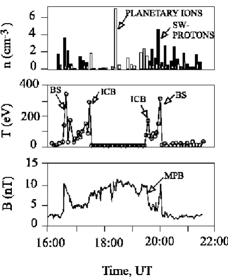
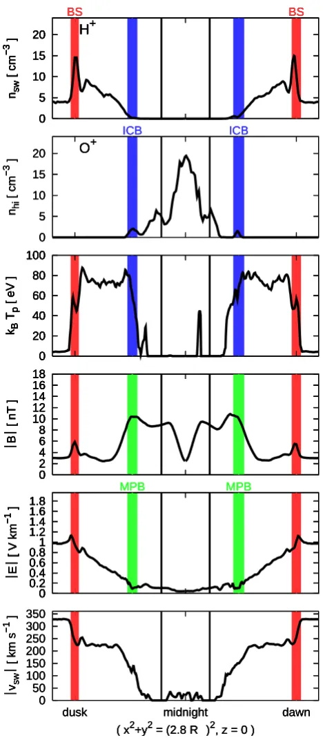
Fig. 1. Number density of the solar wind protons and heavy ions, proton temperature and magnetic field along a circular orbit from 16 March 1989 measured by ASPERA on board Phobos-2 (adapted from Sauer and Dubinin, 2000). In the plasma wake of the planet no solar wind protons are observed (proton cavity). The ion com-position boundary (ICB) separates the solar wind protons from the planetary ions in this orbit. The sharp decrease of the proton tem-perature shows a clear feature of this boundary. At the same position a magnetic pile-up boundary (MPB) can be seen.

showed that at altitudes between 300 and 500 km for a so-lar zenith angle between 75◦_{and 90}◦_{, the energetic electron} flux drops abruptly by nearly one order of magnitude (Acu˜na et al., 1998; Mitchell et al., 2000). This feature was termed PEB by Crider et al. (2003) and it was identified as the loca-tion of the ionopause (Mitchell et al., 2001). From this, the height of this boundary at the subsolar point can be estimated to be 150–200 km. Furthermore, cold electrons above this boundary were observed by MGS (Acu˜na et al., 1998). These cold electrons may indicate the presence of clouds or stream-ers of cold ionospheric plasma detaching from the ionopause, as it was observed at Venus (Brace et al., 1982).

MGS, as well as the Phobos-2 MAGMA instrument, de-tected an additional feature in the magnetic field structure, the so-called magnetic pile-up boundary (MPB), as reported by Riedler et al. (1991) and Vignes et al. (2000). The MPB is localized between the bow shock and the ionopause/PEB. The magnetic field vector rotates, its mean amplitude begins to increase, fluctuations are reduced, and energetic electron fluxes begin to decrease. The same structures have been ob-served at active comets like Halley and Grigg-Skjellerup by the Giotto mission (Mazelle et al., 1989; R`eme et al., 1993),

as well as at Venus (Bertucci et al., 2003). Ion measurements by the ASPERA and TAUS experiments on board Phobos-2 also identified an ion composition boundary (ICB) nearly at the same position as the MPB which separates the so-lar wind protons from the planetary ions (Rosenbauer et al., 1989; Breus et al., 1991; Sauer et al., 1994). Figures 1 and 2 show data from Phobos-2 orbits (Lundin et al., 1989; Grard et al., 1989; Riedler et al., 1989; Sauer et al., 1990), which exhibit the described features. Furthermore, Phobos-2 mea-surements also detected several energetic beam structures in-side the plasma tail of Mars formed by the planetary ions (Lundin et al., 1990).

To gain an insight into the physics of these structures, sev-eral different numerical investigation have been carried out. MHD studies by Liu et al. (2001) showed good agreement of the positions of the bow shock and the ionopause with the MGS results. However, in this model all ion species have the same velocity and temperature. The effects of finite ion gy-roradii, like asymmetries and different ion accelerations, are not taken into account. The ICB could not be reproduced by MHD models.

An important improvement of the general MHD approach is the bi-ion fluid model frequently used by Sauer and Du-binin (2000). In this model, two distinct fluids are used for the solar wind protons and the planetary ions, taking the large gyroradius of the planetary ions into account.

Sauer et al. (1992) and Baumg¨artel and Sauer (1992) showed that for the subsonic flow behind the bow shock, there exist critical points, where stationary, spatially con-tinuous mass loading is no longer possible. These criti-cal points are the “generalized sonic points” in a two-fluid plasma (McKenzie et al., 1993) and may occur already in re-gions where the planetary ion densitynhibecomes

compara-ble to the solar wind proton densitynsw. According to Sauer

and Dubinin (2000) this may result in a sudden stoppage of the proton flow and the formation of a “proton cavity” around the obstacle. This “obstacle boundary” at Mars does not co-incide with the ionopause, where the stagnation of the flow could be expected. The “obstacle boundary” is character-ized by a change in the ion composition and the pile-up of the magnetic field. The magnetic field frozen in the electron flow is carried across this boundary and piled up due to the decrease of the electron velocity which is adjusted to a driven slow motion of the heavy planetary plasma in the boundary layer between the obstacle boundary and ionopause.

Because of the finite gyroradius of the solar wind protons, which is of the order of the characteristic length scales of the simulation region, a kinetic treatment seems mandatory. However, a fully kinetic approach is not feasible with current computational resources. Therefore, a hybrid model, where the ions are treated as particles, and the electrons are treated as a fluid, is used here.

barrier in front of the planet with asymmetries along the so-lar wind electric field, a magnetotail, and a few tail structures. Kallio and Janhunen (2001) used a hybrid model to study the atmospheric effects of proton precipitation in the atmosphere and the ion escape at the nightside of the planet (Kallio and Janhunen, 2002). In this model an exospheric ion source was included. These simulations also showed a magnetic pile-up, but well-defined boundaries are not to be seen.

Kallio and Janhunen (2002) do not include an electron pressure term at all, whereas Shimazu (2001) uses a global electron pressure gradient for the solar wind plasma and the planetary ions plasma. However, Hanson and Mantas (1988) showed the presence of three different electron populations with different temperatures. Hence, it is desirable to treat the electron pressure inside the ionosphere differently from that of the solar wind.

We use a newly-developed hybrid model with a detailed quantitative model for the planetary ion densities, which in-cludes two electron fluids with different temperatures, as well as a friction force between ions an neutral gas atoms (Bagdonat and Motschmann, 2002a).

2 Model and parameters

2.1 Basic equations

The numerical investigations are done using a new hybrid code by Bagdonat and Motschmann (2002a). In the hy-brid approximation the electrons are modeled as a massless charge neutralizing fluid, whereas the ions are treated as in-dividual particles. The time integration scheme of this code is based on that introduced by Matthews (1994). The code is able to use an arbitrary, curvilinear grid in up to three spa-tial dimensions. This feature is used here to enhance the resolution near the Martian surface and to adapt to the Mar-tian sphere. The actual form of the grid used is described in Sect. 2.3. The numerical details for handling a curvilinear grid are based on the scheme introduced by Eastwood et al. (1995) and described in Bagdonat and Motschmann (2002a). A collisional force between ions and ionospheric neutral gas atoms (neutral drag force) is included to take into account possible collisional effects.

For the ions, the equation of motion

dvs

dt =

qs

ms

(E+vs×B)−kDnn(vs −un) (1)

is solved, where whereqs,ms andvs are the charge, mass and velocity of an individual particle of speciess, respec-tively;nn andun are the number density and bulk velocity of the neutrals. The neutral gas density distribution will be described in detail below; kD is a constant describing the collisions of ions and neutrals, given as 1.7·10−9cm3s−1by Israelevich et al. (1999). From the momentum conservation of the electron fluid the electric field can be derived as

E= −ue×B−

∇pe,sw+ ∇pe,hi

ρc

, (2)

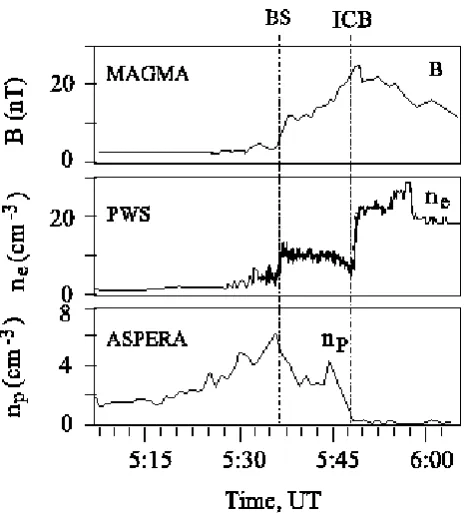
Fig. 2. Data obtained from different instruments on board Phobos-2 along an elliptical orbit from 8 February 1989 (adapted from Sauer and Dubinin, 2000). The ion composition boundary is recognized by a sharp increase in the electron density which indicates the iono-spheric plasma and a decrease of the solar wind density. The mag-netic field piled up until this position. The decrease of the proton density downstream of the BS probably results from a somewhat small angle of view of the ASPERA instrument.

whereue denotes the electron bulk velocity, computed from the ionic currents and the overall currents by means of

ue=

Jion

ρc

−∇ ×B

µ0ρc

, (3)

where ρc is the overall charge density of the ions and the electrons due to quasi-neutrality.

We use two different electron pressure terms in Eq. (2) to take into account the different electron temperatures of the solar wind and ionospheric electrons, respectively. Hanson and Mantas (1988) and Johnson and Hanson (1991) have obtained the presence of several electron populations with different temperatures from Viking measurements, justify-ing the above assumption. Both electron populations are as-sumed to be adiabatic, i.e.

pe,sw/hi=βe,sw/hi

_n

e,sw/hi

n0

κ

(4) with two different temperatures given byβe,swandβe,hifor

z

y

x

B

v

E

X

Y

Z

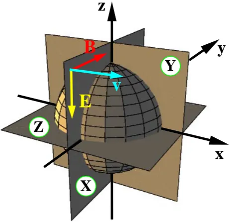
Fig. 3. Cross sections of the simulation box at the planex=0,y=0 andz=0 presented in Sect. 4.

same for the electrons as the corresponding ion number den-sities, because of quasi-neutrality. An adiabatic exponent of κ=2 was used instead of 5/3, because the thermodynamic coupling is only effective in the two dimensions perpendicu-lar to the field.

For the time evolution of the magnetic field one obtains from Farady’s law

∂B

∂t = ∇ ×(ue×B) . (5)

Further on, a magnetic diffusivity is realized in the code by a 3-D 27-point smoothing procedure.

2.2 Parameters

In the standard run the upstream solar wind parameters are as follows: the undisturbed density of the solar wind protons nsw,0=4 cm−3, the undisturbed bulk velocity is

vsw,0=10 VA0 with the Alfv´en velocity VA0=32.7 km s−1

and the undisturbed interplanetary magnetic field (IMF) amounts toB0=3 nT. The Larmor radiusvsw,0/ ci of the

shocked solar wind protons can reach values of several hun-dred kilometers and thus it is comparable to the size of the interaction region. For oxygen ions the Larmor radius would be several thousand kilometers and hence larger than the typ-ical length scales.

WhereasTe,sw≈2·105K is well known from temperature

measurements (Pilipp et al., 1990), a critical, unknown pa-rameter isTe,h, the electron temperature of the ionospheric

ions. These electrons are produced by EUV ionization. The retarding potential analyzers (RPAs) carried on board the two Viking Landers (Hanson et al., 1977) provided informa-tion on the ion and electron temperatures for a limited alti-tude range and along two profiles in the northern hemisphere

(Hanson and Mantas, 1988). They found three coexisting electron gases. Above 200 km, the high-energy electrons with a number density of the order of 10 cm−3_{is probably}

of solar wind origin. The medium energy population has a peak value of 600 cm−3 at 140 km withTe≈20 000 K.

Be-tween 300 and 140 km the density of the “cold” ionospheric population with a temperature around 3000 K increases and reaches its peak of about 105cm−3 near 140 km. Below 200 km, where the thermal coupling to the ions and neutral gas atoms dominates over heat transport processes, the tem-perature of the “cold” population decreases, and reaches the neutral gas temperature (100–200 K) at about 120 km.

Three different electron temperatures were tested for the ionospheric electrons in order to study the effects of this temperature parameter: an “increased” temperature Te,h=100 000 K which is almost equal to the solar wind

temperature, a “medium” temperatureTe,h=20 000 K and a

“low” temperatureTe,h=3000 K.

2.3 Simulation geometry

In all runs the simulation box has three spatial dimen-sions, with the undisturbed solar wind flowing in the pos-itive x-direction, and the undisturbed interplanetary mag-netic field being oriented perpendicular in the positive y-direction. The convective electric field E=−v×B points therefore to the negative z-direction (see Fig. 3). The hemi-sphere to which the electric field is pointing is denoted as the E+hemisphere, the other as E−hemisphere. In the ge-ometry used here, these would be the southern and north-ern hemispheres, respectively. The size of the simulation box is−2RM≤x, y, z≤2RM, whereRM is the Martian

ra-dius. For studying the tail structures a larger box with

−3RM≤x, y, z≤3RMis used.

It is useful to have a grid structure with adapted resolu-tion to resolve the different scales for the ionosphere and the much larger bow shock. The adaptive grid of Ma et al. (2002) has proven to be a very good choice to accomplish this. How-ever, in a particle code this method is far more complicated due to the fact that in smaller cells fewer particles will also be located, thereby introducing much noise in the region of high resolution. This may be overcome by means of some parti-cle splitting and coalescence techniques, such as described in Coppa et al. (1996), Lapenta and Brackbill (1994) and Kallio and Janhunen (2002). Actually, our code is capable of some basic coalescence technique, but for the runs presented here, this method turned out to be unsuited.

In order to adapt the grid to the Martian sphere and to en-hance the resolution in the vicinity of the planetary surface, a grid like that in Fig. 4 was used. A 3-D Cartesian grid with the origin in the center and a box dimensionLx, Ly, Lz is divided intoNx×Ny×Nz grid cells. rij k is the location of the grid nodei, j, k, wherei, j, k=0, . . . , Nx, Ny, Nzand

rij k=(exLx/2, eyLy/2, ezLz/2)with

e_{ij k} = ex, ey, ez

= 2i/Nx−1,2j/Ny−1,2k/Nz−1

2

1

0

-1

-2

2 1

0 -1

-2

z(R

M

)

x(R ) 2

1

0

-1

-2

2 1

0 -1

-2

z(R

M

)

x(R )

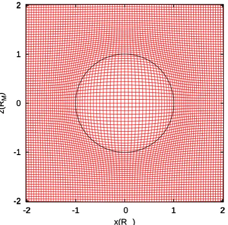
Fig. 4. Structure of the simulation grid used. A cross section through the box is shown withα=0.21,β=0.37 andγ=7.07 (see text) consisting of 80×80 cells in the planey=0. This grid used for the actual simulation runs, gives a higher resolution near the Mar-tian surface (black circle) compared to the outer cells.

The grid of Fig. 4 is constructed by stretching these positions by

r0_{ij k} =rij k·

"

1+ α/β

1+exp

(|eij k| −β)γ

#

, (6)

whereαis a parameter describing the amount of deformation andγ denotes the width of the deformation around Mars. The parameterβ marks the radius of the maximum resolu-tion. The resulting grid is obviously not orthogonal.

Simulating with this grid one obtains the highest resolu-tion of about 100 km/cell near the surface. The cells outside the planet never become larger than 170 km.

The boundary conditions are a critical point. At the left-hand side of the simulation box, the solar wind comes in (in-flow boundary), whereas at the right-hand side it leaves the box (outflow boundary). For the remaining sides some sort of free or absorbing boundary is desirable, however, that turned out to make the simulations unstable. We therefore use in-flow boundary conditions, which simply keep the field values constant. The “inner” boundary at the planetary surface will be dealt with in Sect. 3.1.

3 Ionospheric model

Each simulation run starts without the planetary atmosphere. The atmosphere is then “switched on”, i.e. a certain amount of neutral gas density per time unit is produced. The situation evolves until a quasi-stationary state is reached.

108

107

106

105

104

103

102

101

3000 2000 1000

500 300 150

1017 1016 1015 1014 1013 1012 1011 1010 109 108

ion production rate [m

-3 s -1]

neutral density [m

-3]

Altitude [km]

neutral profile ion production profile (subsolar) ion production profile (terminator)

Fig. 5. Neutral gas density (blue line), the ion production rate (red line in subsolar direction and green line at the terminator) of oxygen as a function of altitude at solar minimum (ν=1·10−7s−1). Note the two different axis scales.

The Martian atmosphere is modeled as a spherical sym-metric gas cloud around Mars, consisting of atomic oxygen. The radial density distribution contains an ionospheric expo-nential profile and an exospheric 1/rprofile for the oxygen corona above 500 km. To take into account the measured small deviations from the inner exponential behaviour, we use two exponential terms with different scale heights, i.e.

nn(r)=n1 exp

r₁−r

H1

+

n2exp

r₂−r

H2

+n3

r3

r . (7)

The parameters have been obtained from a fit to data given by Chen et al. (1978), Kallio and Luhmann (1997) and Ko-tova et al. (1997) for solar minimum conditions. The result-ing values aren1=3·1014m−3,r1=140 km,n2=2·1011m−3,

r2=300 km, n3=1·109m−3, r3=1700 km, H1=27 km and

H2=35 km. The resulting neutral gas density using these

val-ues is plotted as a blue line in Fig. 5.

At distances below 180 km above the Martian surface, the predominant constituent is CO2(Chen et al., 1978), but

mix-ing of O and CO2would not change the basic physical

prop-erties of our results.

For constant solar UV radiation one obtains the ion pro-duction rate withnn(r)from Eq. (7) to be

∂ni(r, χ )

∂t =ν κ nn(r)·

exph− σ cos(χ )

n

n1H1·exp

r₁−r

H1

+

n2H2·exp

r₂−r

H2

+n3r3·log(RM/r)

oi

, (8)

ion production rate [106 m-3 s-1]

300 250

200 150

Altitude [km]

+π/2 +π/4 0 -π/4

-π/2 SZA 10

8

6

4

2

0

Fig. 6. Ion production rate of oxygen as a function of altitude and solar zenith angle (SZA) at solar minimum.

parameter fitted to the position of the ion production maxi-mum of 150 km given by Krasnopolsky (2002). From this fitσ=1.8·10−19_m2_{was obtained;κ=1 is here the ionization}

efficiency. The resulting ion production rate is illustrated in Fig. 5 (red and green line) and Fig. 6.

For most of the simulation runs the value of the ionization frequencyν was adapted to the conditions met by Phobos-2 and MGS to compare the results to their measurements. Note that the mission Phobos-2 was during solar maximum (ν≈3·10−7s−1), Viking at solar minimum (ν≈1·10−7s−1) and MGS made measurements, as the solar activity increased from solar minimum toward solar maximum. The ionization frequencies are taken from Zhang et al. (1993) and Bauske et al. (2000).

For increasing solar zenith angle the position of the max-imum ionization rate increases from 150 km atχ=0 (sub-solar) up to 260 km atχ=π/2 (terminator). The peak rate at the terminator line drops off to 10% of the subsolar max-imum rate (see Figs. 5 and 6). At the terminator line and at the whole nightside of the planet a constant ion produc-tion funcproduc-tion∂ni/∂t was assumed, yielding about 10% of the dayside production rate. Equation (8) cannot be applied for the nightside. Other ion production processes, like elec-tron impact ionization and charge exchange, are not included in our model.

3.1 Inner boundary

All particles, whether planetary ions or solar wind protons are deleted, when hitting the Martian surface. Consequently there are no ion currents inside of Mars. The simulation starts without any magnetic or electric fields in the solid body. Dur-ing the simulation, penetration of the magnetic field through the ionosphere into the solid is allowed. The magnetic diffu-sion is accompanied by the penetration of the electric field. Thus the interior of Mars is not completely field free.

To avoid a collapse of the ionosphere through the inner boundary (surface) the solid body is approached by an ho-mogeneous heavy ion density without any movement of the ions. Alternative inner boundary conditions were studied by Brecht (1997). He assumed a perfect conducting sphere to model the ionosphere. Heavy Martian ions are not included and thus the ICB may not be described.

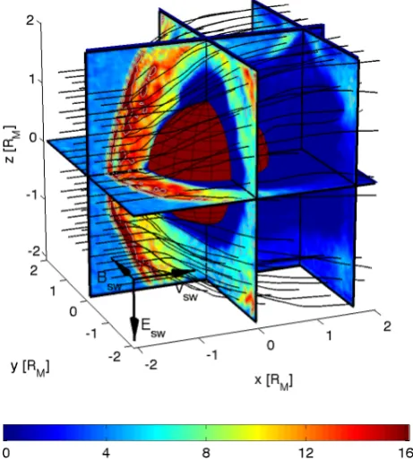
Fig. 7. Simulation results for the “standard run”. The cutting planes show the solar wind density in cm−3. The black solid lines repre-sent streamlines of the corresponding velocity field. The solar wind flows almost symmetrically around the obstacle. On the nightside, a plasma wake is formed, where the solar wind density vanishes al-most completely. This wake region, however, is not symmetric with respect to the equatorial plane, as can be seen from the cutting plane atx=5/3RM. Downstream of the bow shock, a multiple shocklets structure is obvious.

Parameters: t=1392 s,ν=2·10−7s−1(medium solar conditions), Te,h=2·104K (medium temperature),nsw=4 cm−3,Bsw=3 nT.

4 Results

The accessible data for a simulation run are the density, bulk velocity and thermal velocity of the solar wind protons and the planetary O+_{-ions, respectively. The electron data of the} fluid can be deduced from the ion data due to quasi-neutrality and they contained the density, bulk velocity and mean tem-perature. These are accompanied by the magnetic and elec-tric field data. We performed one simulation, denoted as “standard run”, using the parameters given in Sect. 2.2 with the medium temperatureTe,h=20 000 K for the ionospheric

electrons and the ionization frequencyν=2·10−7s−1. Us-ing this value in Eq. (8) yields a total ion production rate of Q=5.37·1025s−1. This set of parameters corresponds to av-erage solar conditions.

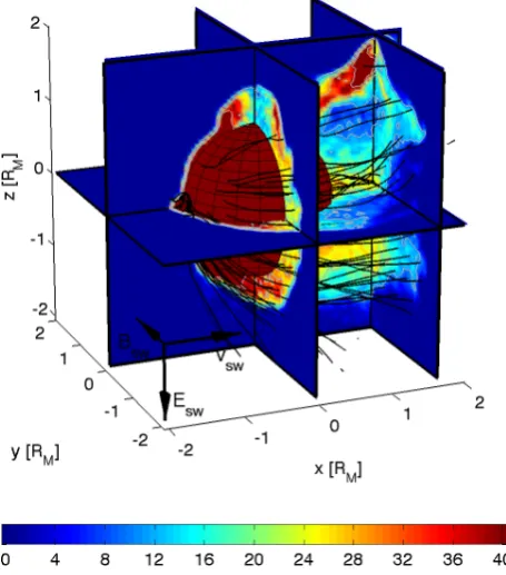
Fig. 8. Simulation results for the “standard run” continued. The cutting planes show the heavy ion density (O+) in cm−3. The black solid lines represent the streamlines of the corresponding ve-locity field. The heavy ions form a complex tail structure behind the planet. Note the boundary on the dayside, where the heavy ion density shows a sharp increase. This is also the case for the upper edge of the ion tail in the E− hemisphere (above the north pole), whereas in the E+hemisphere the boundary is not that pronounced. If one compares this to Fig. 7, the sharply bounded tail fits exactly into the solar wind plasma wake. Hence, both ion species are com-pletely separated. This boundary is the “ion composition boundary” (ICB). Inside the tail the heavy ion density becomes asymmetric, as is seen at the planex=5/3RM. The heavy ions form rays inside the tail. The flow pattern is much more asymmetric with respect to the equatorial plane compared to the solar wind flow pattern. Beneath the south pole some cycloidal motion of a large gyroradius can be seen, whereas in the rest of the tail region the stream lines are bun-dled inside the tail rays. Furthermore, a wave-like structure with rather large amplitude is evolved on the dayside at the ICB in the E−hemisphere (north pole). This wave strips off heavy ion plasma clouds with high density. This structure is non-stationary.

Parameters: see Fig. 7.

equatorial plane, are given to compare these standard results with the data measured by Phobos-2. Figure 13 shows two further one-dimensional cuts at 850 km above the north and below the south pole in the polar plane to illustrate the asym-metric behaviour of the ionosphere.

Finally, the ionospheric electron temperature, the solar wind ram pressure, and the ionospheric production rate are varied to study their influence on the various plasma bound-aries’ positions. The results are compiled in Sect. 4.3.

Fig. 9. Simulation results for the “standard run” continued. The cut-ting planes show the magnetic field in nT. The black solid lines rep-resent the magnetic field lines. The magnetic field lines are draped around the obstacle. Just in front of the ICB, the magnetic field reaches its maximum, which indicates the “magnetic pile-up bound-ary” (MPB). The magnetic field vanishes inside the wake in the po-lar plane. The full three-dimensional structure in the tail is again highly asymmetric and complicated. The same shocklet substruc-turing as in Fig. 7 can be seen downstream of the BS.

Parameters: see Fig. 7.

4.1 Global 3-D views

Three global 3-D views of the standard run results are shown in Figs. 7–9 for the solar wind density, the heavy ion density and the magnetic field configuration, respectively. The cut-ting planes through the simulation box are taken at the planes x=0,x=5/3RM,y=0 andz=0. Note that the stream lines in

Figs. 7 and 8 indicate the direction of the plasma bulk flow, but do not necessarily coincide with the trajectories of the individual particles.

Figure 7 shows an almost symmetric flow of the shocked solar wind around the obstacle. Behind the obstacle, a plasma wake is formed, where the solar wind density almost vanishes (proton cavity). Furthermore, shock substructures, which were called “shocklets” by Omidi and Winske (1990) or also referred to as “multiple shocks” by Shimazu (2001) can be seen in the downstream region of the bow shock. A more detailed description of these structures will be given in Sect. 4.2.

0 2 4 6 8 10 12 14 16 n_sw [ cm−3 ]

B_sw sw z(R M ) 3 2 1 0 −1 −2 −3

y(R_M) 3 2 1 0 −1 −2 −3 1 10 n_hi [ cm−3 ]

3 2 1 0 −1 −2 −3

y(R_M) 3 2 1 0 −1 −2

−3 0

2 4 6 8 10 12 14 16 18 B [ nT ]

3 2 1 0 −1 −2 −3

y(R_M) 3 2 1 0 −1 −2 −3 0 2 4 6 8 10 12 14 16 v_sw sw

n_sw [ cm−3 ]

z(R M ) 3 2 1 0 −1 −2 −3 3 2 1 0 −1 −2 −3 1 10 n_hi [ cm−3 ]

3 2 1 0 −1 −2 −3 3 2 1 0 −1 −2

−3 0

2 4 6 8 10 12 14 16 18 B [ nT ]

3 2 1 0 −1 −2 −3 3 2 1 0 −1 −2 −3 0 50 100 150 200 250 300 350 vsw [ km s−1 ]

z(R M ) 3 2 1 0 −1 −2 −3

x(R_M) 3 2 1 0 −1 −2

−3 0

50 100 150 200 vhi [ km s−1 ]

3 2 1 0 −1 −2 −3

x(R_M) 3 2 1 0 −1 −2

−3 0

0.2 0.4 0.6 0.8 1 1.2 1.4 1.6 1.8 E [ V km−1 ]

3 2 1 0 −1 −2 −3

x(R_M) 3 2 1 0 −1 −2 −3 0 2 4 6 8 10 12 14 16 v_sw sw

n_sw [ cm−3 ]

y(R M ) 3 2 1 0 −1 −2 −3 3 2 1 0 −1 −2 −3 1 10 n_hi [ cm−3 ]

3 2 1 0 −1 −2 −3 3 2 1 0 −1 −2

−3 0

2 4 6 8 10 12 14 16 18 B [ nT ]

3 2 1 0 −1 −2 −3 3 2 1 0 −1 −2 −3 0 50 100 150 200 250 300 350 v_sw [ km s−1 ]

y(R M ) 3 2 1 0 −1 −2 −3

x(R_M) 3 2 1 0 −1 −2

−3 0

50 100 150 200 v_hi [ km s−1 ]

3 2 1 0 −1 −2 −3

x(R_M) 3 2 1 0 −1 −2

−3 0

0.2 0.4 0.6 0.8 1 1.2 1.4 1.6 1.8 E [ V km−1 ]

3 2 1 0 −1 −2 −3

x(R_M) 3 2 1 0 −1 −2 −3 3 2 1 0 −1 −2 −3 3 2 1 0 −1 −2 −3 3 2 1 0 −1 −2 −3 3 2 1 0 −1 −2 −3 3 2 1 0 −1 −2 −3 3 2 1 0 −1 −2 −3 3 2 1 0 −1 −2 −3 3 2 1 0 −1 −2 −3 3 2 1 0 −1 −2 −3 3 2 1 0 −1 −2 −3 3 2 1 0 −1 −2 −3 3 2 1 0 −1 −2 −3 3 2 1 0 −1 −2 −3 3 2 1 0 −1 −2 −3 3 2 1 0 −1 −2 −3 3 2 1 0 −1 −2 −3 3 2 1 0 −1 −2 −3 3 2 1 0 −1 −2 −3 3 2 1 0 −1 −2 −3 3 2 1 0 −1 −2 −3 3 2 1 0 −1 −2 −3 3 2 1 0 −1 −2 −3 3 2 1 0 −1 −2 −3 3 2 1 0 −1 −2 −3 3 2 1 0 −1 −2 −3 3 2 1 0 −1 −2 −3 3 2 1 0 −1 −2 −3 3 2 1 0 −1 −2 −3 3 2 1 0 −1 −2 −3 3 2 1 0 −1 −2 −3

(a)

(b)

(c)

(d)

(e)

(f)

(g)

(h)

(i)

(j)

(k)

(l)

(m)

(n)

(o)

X

Y

Z

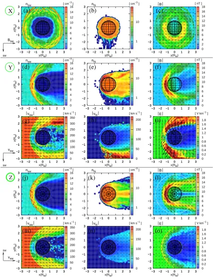
Fig. 10. Simulation results for the “standard run” for three orthogonal cross sections through the simulation box. (a), (d), (j) solar wind density, (b), (e), (k) heavy ion density, (c), (f),(l)magnetic field and vectors, (g), (m) solar wind bulk velocity, (h), (n) heavy ion bulk velocity and (i), (o) electric field, for the respective cutting planes from Fig. 3. The white lines in panel (l) correspond to the one-dimensional cuts of Figs. 11 and 12. The density plots show a clear separation of solar wind ions and heavy ions (ICB). The convective electric field

E=−v×B vanishes, where the plasma of the heavy ions dominates. The magnetic field piles up at the planet’s dayside and reaches a maximum value (MPB), where the ICB is located. On the nightside the slow, heavy ions form several rays; below the south pole a fast component of pick-up ions is present. The bow shock exhibits some shocklet substructuring. See text for details.

The ICB is very sharp at the dayside of the planet and along the whole edge of the tail in the E−_{hemisphere (above the} north pole), whereas this boundary in less pronounced in the E+hemisphere (below south pole). The proton wake is filled inhomogenously with ionospheric plasma, and the heavy ion density is highly asymmetric (see the plane x=5/3RM in

Fig. 8). Several more or less distinct “rays” of high heavy ion density are formed inside the tail, which is in accor-dance with the results of Lichtenegger and Dubinin (1998). Below the south pole the flow is dominated by a cycloidal particle motion with large gyroradius (heavy pick-up ions). This pickup is similar to that at weak comets (Bagdonat and Motschmann, 2002b; Bogdanov et al., 1996). Inside the tail the electric field carried by the solar wind vanishes, as will be shown in the next section. Therefore, the heavy ions inside the tail gyrate with a much smaller gyroradius.

A wave-like structure can be seen in the vicinity of the ICB above the north pole. Heavy ion plasma clouds with high density are stripped off from the dayside ICB region and carried over the north pole towards the tail. This is probably caused by a Kelvin-Helmholtz instability (Wolff et al., 1980; Luhmann and Bauer, 1992) or some other electromagnetic LF wave generation.

Figure 9 shows the typical magnetic field configuration with the field lines draping around the obstacle. Due to this draping, the magnetic field is increased in front of the ob-stacle. The maximum value is reached just in front of the ICB, indicating the presence of a “magnetic pile-up bound-ary” (MPB). The same behaviour can be seen at the displaced heavy ion cloud nearx=5/3RM,y=2RM, where the

mag-netic field is increased in front of the high heavy ion density. On the nightside, the magnetic field lines exhibit a mul-tiply curved form, corresponding to the ray structure in the heavy ion density. In the equatorial plane and in the plane x=5/3RM, a magnetic field lobe can be seen, which of

course is also present on the opposite side. Between the two lobes, the magnetic field is strongly decreased in the polar plane.

4.2 2-D and 1-D cuts through the simulation box

Figure 10 shows two-dimensional cuts of the 3-D results from the standard run at the cutting planesx, y, z=0, which are denoted by X, Y, Z, respectively, as indicated in Fig. 3. The cuts show data from a stationary state att=1169 s, which is somewhat earlier compared to the 3-D views. This time corresponds to a duration, in which the undisturbed solar wind protons would cross the whole box (4RM) 28 times.

This large simulation time is mandatory, because of the slow movement of the heavy ions behind the planet.

The multiple shocklet structure can be seen particularly in the solar wind density and electric field in the polar plane (Figs. 10d, i). This structuring is due to the finite gyrora-dius of the solar wind protons, and was already described by Omidi and Winske (1990) and Shimazu (2001). The charac-teristic scale of these shock substructures is determined by the width of the cycloidal motion. The gyroradius of the

shocked solar wind protons at the line sun-planet (B⊥vsw)

withvsw≈100 km s−1andB≈12 nT is

rg=

mvsw

eB ≈90 km. (9)

From this, the characteristic scale follows as 2π rg≈550 km. This estimate agrees well with the results in Fig. 10. Thus, the shocklet structuring is essentially kinetic.

As can be seen from Fig. 10a and also Fig. 17a, the bow shock is not circular at the terminator plane. This is due to the dependence of the propagation velocity of the fast magne-tosonic wave on the angle between the propagation direction and the IMF. Furthermore, the bow shock is also asymmet-ric with respect to the equatorial plane. This asymmetry is caused by a reduction in the downstream fast mode veloc-ities due to the mass-loading by the escaping oxygen ions. The ionopause cannot be seen in these 3-D simulation runs, because the numerical diffusion is too large.

The comparison of the solar wind density and the heavy ion density plots for all cutting planes in Fig. 10 clearly ex-hibits the ICB boundary. The solar wind velocity fields in Figs. 10g and m show that the solar wind always flows par-allel to the ICB. Only a very small portion of fast solar wind crosses the ICB, which then contributes to the thin region of high velocity at the ICB. As stated by Sauer et al. (1992), the solar wind protons are accelerated due to the transition from sub- to supersonic flow, when crossing the ICB. This is in agreement with our results. However, the significant drop in the SW density is not due to this acceleration, but simply caused by the deflection of the solar wind due to the electric shock potential at the bow shock and the strong electric field due to the electron pressure gradient of the heavy ion plasma component at the ICB.

The MPB can be seen from Figs. 10f andl. In the vicinity of the subsolar region, where the heavy ion plasma is almost at rest (see, e.g. Figs. 10h and n), the magnetic field is mainly transported beyond the ICB by diffusion and not by convec-tion. Therefore, the MPB is located at the same position as the ICB. The magnetic field cannot penetrate the areas with high heavy ion density. In the tail region, where the heavy ions have already reached some finite velocity, the magnetic field is also convected by the heavy ion plasma. This forms the two lobes, as can be seen from Fig. 10l.

(2003) and was simulated by Brecht (1997), Shimazu (2001) and Kallio and Janhunen (2002). In the equatorial plane (see Figs. 10j–o), the situation is symmetric.

The global configuration of the draped magnetic field lines can be seen from Fig. 9. The curvature, as well as the mag-netic field gradients, exert a magmag-netic tension and a pressure force on the SW protons and the heavy ions. These forces are strongest in the vicinity of the poles, where the draped field lines can unwind. Figure 10g shows that it results in an acceleration of the solar wind above the north pole. The same accelerating force is compensated by the slowing down of the SW due to the mass-loading below the south pole.

The heavy ions react on this force similarly, being dragged towards the tail. As can be seen from Fig. 10h, the acceler-ation of the heavy ions is strongest near the ICB, where the field lines can penetrate the heavy ion plasma. However, the heavy ions remain significantly slower compared to the solar wind ions.

The parallel flow of both components with different veloc-ities at the ICB could excite a Kelvin-Helmholtz-instability (Wolff et al., 1980; Luhmann and Bauer, 1992), which forms a wave with a rather large amplitude. This can indeed be seen from Fig. 10 and especially Fig. 15b. At some times large ionospheric plasma clouds are stripped off the ionosphere and become strongly accelerated, as is seen in Figs. 10e and h. In the E+hemisphere this effect does not occur because both ion species are mixed.

An alternative explanation for the case of Venus was given by Shapiro et al. (1995). A modified two-stream lower hybrid instability could be responsible for this kind of wave excita-tions and momentum exchange between the shocked solar wind. As a result of this interaction, the planetary plasma becomes heated and accelerated outside of the ionosphere, close to the upper boundary of the ionopause. Planetary ions can be dragged away by the solar wind flow, thereby leaving the planetary magnetosphere.

The heavy ion tail on the nightside exhibits some ray struc-turing. Generally, the heavy ion density is higher, where the magnetic field is lower, so that the pressure balance is re-tained. The pronounced region of lower magnetic field be-tween the two lobes in the polar plane, as can be seen in Figs. 10f andl, gives rise to the central main ion tail (plasma sheet) (see, e.g. Figs. 10e and k). The origin of the other tail rays on either side from the central tail ray in the equatorial plane (Fig. 10k and Fig. 16c) is not yet completely clear.

Figure 11 shows a one-dimensional cut parallel to the x-axis aty=−1.25RM (850 km above the surface) and z=0

(white line in Fig. 10l). The data is taken as an average dur-ingt=1127−1197 s. The figure should be compared to the measurements of Phobos-2 shown in Fig. 2. The magnetic field reaches a value of about 20 nT at the MPB in our sim-ulation results, which is in good quantitative agreement with the data obtained by the MAGMA instrument on Phobos-2. The electron density is also in good qualitative agreement; note, in particular, the ratio of the density jumps at the BS and the ICB. Furthermore, the local minimum in the vicin-ity of the ICB is reproduced in our results. However, the

proton density measured by ASPERA (Fig. 2) shows a pro-nounced foot region, which cannot be seen from Fig. 11. Phobos-2 crossed the bow shock near the subsolar point at 1.5RM, where the angle between the IMF and the shock

nor-mal was about 57◦(Schwingenschuh et al., 1990). The solar wind parameters were vsw=450 km s−1 andnsw=1.7 cm−3

(Szeg¨o et al., 1998), which is half of the proton density in the simulation. For the cut in Fig. 11, the angle between the IMF and the shock normal is about 75◦. Therefore, the foot region does not occur in our results. The decrease ofnp in the ASPERA measurements at the BS is probably due to the constrained view of direction of the instrument (Szeg¨o et al., 1998).

A few high energetic solar wind protons, which are not reflected, cross the ICB and no longer feel the electric field

Esw=−vsw×B. They react only on the Lorentz force and

turn round in the z-direction (see Fig. 11 and Fig. 17b). Figure 12 shows the simulation results along a circular or-bit withr=2.8RM. These should be compared to the circular

orbit of the same size of Phobos-2 in Fig. 1. The simula-tion results show that the planetary ions are split up into the central tail (plasma sheet) with high density and several rays with smaller density (see also Fig. 16c). The planetary ions tend to accumulate where the magnetic field has local min-ima. This was also found at MHD simulations by Tanaka and Murawski (1997). A similar correlation between the heavy ions and the magnetic field can be seen from the data mea-sured by Phobos-2 (Fig. 1). The reason for this tendency is simply the pressure balance between the thermal pressure of the planetary ions and the magnetic field pressure. The anti-correlation hints towards an excitation of slow mode magne-tosonic waves. The observed magnetic field of about 10 nT in the two magnetic lobes match very well with the simulation results. However, the decrease of the magnetic field between the lobes is much more pronounced in the simulation results compared to the Phobos-2 data at about 18 h 20 min.

In Fig. 12 the proton temperature is also shown. As an additional feature of the ICB, the proton temperature shows a more or less sharp decrease. Inside of the ICB the tem-perature is zero, because there are no protons at all. The av-erage measured temperature in the magnetosheath of about 100 eV matches the simulation results very well. However, the strong overshoot of the temperature at the BS and the ICB is not in accordance with our results. The magnetic field and solar wind velocity jumps at the flank of the BS (Fig. 12) are smaller than in the subsolar region (Fig. 11), because the bow shock becomes quasi-parallel atr=2.8RMin this plane.

0 5 10 15 20

nsw

[ cm

−3

] H

+ BS

0 5 10 15 20

nsw

[ cm

−3

] H

+ BS

0 5 10 15 20

nsw

[ cm

−3

] H

+ BS

0 5 10 15 20 25 30 35 40

nhi

[ cm

−3

]

O+

ICB

0 5 10 15 20 25 30 35 40

nhi

[ cm

−3

]

O+

ICB

0 5 10 15 20 25 30 35 40

ne

[ cm

−3

]

0 5 10 15 20 25 30 35 40

ne

[ cm

−3

]

0 5 10 15 20 25 30 35 40

ne

[ cm

−3

]

0 2 4 6 8 10 12 14 16 18



B



[ nT ]

0 2 4 6 8 10 12 14 16 18



B



[ nT ]

0 2 4 6 8 10 12 14 16 18



B



[ nT ]

0 0.2 0.4 0.6 0.81 1.2 1.4 1.6 1.8



E



[ V km

−1

]

MPB

0 0.2 0.4 0.6 0.81 1.2 1.4 1.6 1.8



E



[ V km

−1

]

MPB

0 0.2 0.4 0.6 0.81 1.2 1.4 1.6 1.8



E



[ V km

−1

]

MPB

0 50 100 150 200 250 300 350

0.0 −0.5

−1.0 −1.5



vsw



[ km s

−1

]

x [ R ] ( y = − 1.25 R , z = 0) dusk 0

50 100 150 200 250 300 350

0.0 −0.5

−1.0 −1.5



vsw



[ km s

−1

]

x [ R ] ( y = − 1.25 R , z = 0) dusk

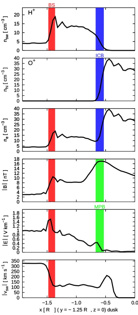
Fig. 11. Simulation results for the “standard run”. Plasma and field parameters along a line parallel to the x-axis in the equatorial plane at

y=−1.25RMandz=0 (straight white line in Fig. 10l). These results should be compared to the measurements made by Phobos-2 in Fig. 2. The figure shows the number density of the solar wind protons and the planetary O+ions, the electron density, the magnetic and the electric field absolute values and the velocity of the solar wind, respectively. The color bars indicate the location of the BS (red), ICB (blue) and MPB (green). The magnetic field and electron density are in good agreement with the observed data. The proton density measured by Phobos-2, however, shows a pronounced foot region, which is not present in our results, due to a differing field geometry described in the text. The interplanetary electric field decreases after the bow shock and vanishes inside of the ICB. However, a small peak just in front of the ICB can be seen. The proton velocity remains constant behind the bow shock but it is increased directly behind the ICB. The very low proton density at this point indicates that only the fastest thermal solar wind protons are able to cross the boundary, leading to this increasing of the bulk velocity. The MPB and ICB are located at the same position, which is in accordance to the Phobos-2 observations.

0 5 10 15 20 nsw [ cm −3 ] H + BS BS 0 5 10 15 20 nsw [ cm −3 ] H + BS BS 0 5 10 15 20 nsw [ cm −3 ] H + BS BS 0 5 10 15 20 nsw [ cm −3 ] H + BS BS 0 5 10 15 20 nsw [ cm −3 ] H + BS BS 0 5 10 15 20 nhi [ cm −3 ] O+ ICB ICB 0 5 10 15 20 nhi [ cm −3 ] O+ ICB ICB 0 5 10 15 20 nhi [ cm −3 ] O+ ICB ICB 0 20 40 60 80 100 kB T p

[ eV ]

0 20 40 60 80 100 kB T p

[ eV ]

0 20 40 60 80 100 kB T p

[ eV ]

0 20 40 60 80 100 kB T p

[ eV ]

0 20 40 60 80 100 kB T p

[ eV ]

0 2 4 6 8 10 12 14 16 18  B 

[ nT ]

0 2 4 6 8 10 12 14 16 18  B 

[ nT ]

0 2 4 6 8 10 12 14 16 18  B 

[ nT ]

0 2 4 6 8 10 12 14 16 18  B 

[ nT ]

0 2 4 6 8 10 12 14 16 18  B 

[ nT ]

0 0.2 0.4 0.6 0.81 1.2 1.4 1.6 1.8  E 

[ V km

−1 ] MPB MPB 0 0.2 0.4 0.6 0.81 1.2 1.4 1.6 1.8  E 

[ V km

−1 ] MPB MPB 0 0.2 0.4 0.6 0.81 1.2 1.4 1.6 1.8  E 

[ V km

−1 ] MPB MPB 0 0.2 0.4 0.6 0.81 1.2 1.4 1.6 1.8  E 

[ V km

−1 ] MPB MPB 0 0.2 0.4 0.6 0.81 1.2 1.4 1.6 1.8  E 

[ V km

−1 ] MPB MPB 0 50 100 150 200 250 300 350 dawn midnight dusk  vsw 

[ km s

−1

]

( x2+y2 = (2.8 R )2, z = 0 ) 0 50 100 150 200 250 300 350 dawn midnight dusk  vsw 

[ km s

−1

]

( x2+y2 = (2.8 R )2, z = 0 ) 0 50 100 150 200 250 300 350 dawn midnight dusk  vsw 

[ km s

−1

]

( x2+y2 = (2.8 R )2, z = 0 )

Fig. 12. Simulation results for the “standard run”. Plasma and field parameters along a circular orbit at 2.8RMaround Mars in the plane

z=0. This should be compared to the data of the circular Phobos-2 orbit in Fig. 1. The black vertical lines mark the crossing of the optical shadow. The colored bars have the same meaning as in Fig. 11. The heavy ion tail is split up in the plasma sheet with high density and four tail rays with smaller densities (see also Fig. 16c). The near midnight rays are located at the minima of the overall magnetic field. This anti-correlation can also be seen from the observed data of Fig. 1. The proton temperature drops down at the ICB, which is also in agreement with Phobos-2 data.

0 5 10 15 20

0.0 −0.5

−1.0 −1.5

[ cm

−3

]

x [ RM ] ( z = 1.25 RM, y = 0 ) north pole

BS ICB

0 5 10 15 20

0.0 −0.5

−1.0 −1.5

[ cm

−3

]

x [ RM ] ( z = 1.25 RM, y = 0 ) north pole

BS ICB

0 5 10 15 20

0.0 −0.5

−1.0 −1.5

[ cm

−3

]

x [ RM ] ( z = 1.25 RM, y = 0 ) north pole

BS ICB

nsw

n_hi

0 5 10 15 20

0.0 −0.5

−1.0 −1.5

[ cm

−3

]

x [ R ] ( z = − 1.25 R , y = 0) south pole BS

0 5 10 15 20

0.0 −0.5

−1.0 −1.5

[ cm

−3

]

x [ R ] ( z = − 1.25 R , y = 0) south pole BS

nsw

n_hi

(a)

(b)

Fig. 13. Cuts along a line parallel to the x-axis in the polar plane at (a)z=1.25RM(850 km above north pole) and (b)z=−1.25RM (850 km below south pole). The ICB, which is clearly developed in the E−hemisphere (a) cannot be seen in the E+hemisphere (b). This results from the different orientation of the electric field in both hemispheres, pointing inwards towards the ionosphere, above the north pole and outwards below the south pole, see also Fig. 10i. Parameters: see Fig. 7.

heavy ion plasma is dragged into the solar wind plasma and the heavy ions are picked up by the solar wind.

In Fig. 14 the total pressure (Ptotal) along the Sun-Mars

line is represented, consisting of kinetic pressure of the solar wind (Pram), thermal pressure of the solar wind (Psw),

ther-mal pressure of the heavy ion plasma (Phi), and magnetic

pressure (PB). We find, as expected, that the total pressure

remains constant. The bow shock is located atx=1.7RM

and the ICB/MPB atx=1.25RM. Note that these values are

larger than in reality because of the higher electron tempera-ture (Te,h=20 000 K) of the heavy ion plasma in this standard

run.

The good quantitative agreement of the simulation results with observed data encourages a closer investigation of the parameter dependence which is done in the next section. 4.3 Parameter study

We investigated the dependence of the position of the ICB on the solar wind density, the production rate of the heavy ions and the electron temperature inside the ionosphere. The left panels in Fig. 16 correspond to the standard run.

Figure 15 shows the influence ofTe,h. The right panels

have a value ofTe,hwhich is five times higher compared to

the left panels. This has basically the effect of “inflating” the heavy ion density, as one would expect. Hence, the ICB is located higher above the planetary surface and the tail struc-turing becomes smoothed. Moreover, the wave instability in the E−hemisphere is more pronounced.

0.01 0.1 1 10

−1.2 −1.4

−1.6 −1.8

pressure [ nPa ]

x [ R ] ( y = 0, z = 0 )

P_sw P_hi P_B P_ram

P_total

Fig. 14. The distribution of the kinetic pressure of the solar wind (Pram), thermal pressure of the solar wind (Psw=Pe,sw+Pi), ther-mal pressure of the heavy ion plasma (P_hi=P_e,hi+P_hi), and magnetic pressure (PB) along the Sun-Mars line on the dayside for the “stan-dard run”.

Parameters: see Fig. 7.

Figure 16 compares the results for two different solar wind densities. The left panels show the results fornsw=4 cm−3,

the right panels fornsw=2 cm−3. Lowering the solar wind

density is in principle equivalent to an increase in the density of the ionosphere. Therefore, the ICB has a larger distance from the surface. The comparison of the left panels of Fig. 15 and Fig. 16 demonstrates the influence of the ionosphere pro-duction rate. In Fig. 16 the propro-duction rate is twice as large as in Fig. 15. Obviously a higher production rate moves the ICB outwards. One can conclude that the electron pressure nekBTe,h inside the ionosphere is the crucial parameter for

the location of the ICB.

We tried to fix this parameter by fitting our results to MGS observational data. The best agreement, shown in Fig. 17, was obtained for a value ofTe,h=3000 K. This temperature

is in good agreement with the measured and most dominant plasma population of the ionospheric O+-ions (Hanson and Mantas, 1988).

The BS and MPB fits in Fig. 17d have been obtained by Vignes et al. (2000) from the MGS observations. Expressed in polar coordinates and assuming a cylindrical symmetry around the x-axis, the equation of the BS and MPB surface is

r= L

1+cos(φ), (10)

where the origin of the polar coordinates is located at (X0,0,0), L is the semi latus rectum and is the

eccen-tricity. The direct fit method of Vignes et al. (2000) yields X0=0.64RM,=1.03,L=2.04RMfor the bow shock, and

X0=0.78RM,=0.9 andL=0.96RM for the MPB,

respec-tively.

5 Summary

1 10

v_sw

sw

n_hi [ cm−3 ]

z(R M ) 2 1 0 −1 −2 2 1 0 −1 −2 1 10

n_hi [ cm−3 ]

2 1 0 −1 −2 2 1 0 −1 −2 1 10 v_sw sw

n_hi [ cm−3 ]

y(R M ) 2 1 0 −1 −2

x(R_M) 2 1 0 −1 −2 1 10

n_hi [ cm−3 ]

2 1 0 −1 −2

x(R_M) 2 1 0 −1 −2 2 1 0 −1 −2 2 1 0 −1 −2 2 1 0 −1 −2 2 1 0 −1 −2 2 1 0 −1 −2 2 1 0 −1 −2 2 1 0 −1 −2 2 1 0 −1 −2

(a)

(b)

(d)

(c)

Y

Z

Fig. 15. Heavy ion distribution around Mars for two different electron tem-peratures inside the ionosphere. (a) and (c)Te,h=2·104K (nominal temp.). (b) and (d) Te,h=1·105K (increased temp.). The ion production rate Qis half of the standard run value. The in-creased temperature for the heavy ions shifts the ICB farther upstream. The tail rays become less sharp. The wave insta-bility in the E−hemisphere above the north pole becomes more pronounced. Parameters: t=1058 s,ν=1·10−7s−1, nsw=4 cm−3.

1 10

v_sw

sw

n_hi [ cm−3 ]

z(R M ) 3 2 1 0 −1 −2 −3 3 2 1 0 −1 −2 −3 1 10 v_sw sw

n_hi [ cm−3 ]

y(R M ) 3 2 1 0 −1 −2 −3

x(R_M) 3 2 1 0 −1 −2 −3 1 10

n_hi [ cm−3 ]

3 2 1 0 −1 −2 −3 3 2 1 0 −1 −2 −3 1 10

n_hi [ cm−3 ]

3 2 1 0 −1 −2 −3

x(R_M) 3 2 1 0 −1 −2 −3 3 2 1 0 −1 −2 −3 3 2 1 0 −1 −2 −3 3 2 1 0 −1 −2 −3 3 2 1 0 −1 −2 −3 3 2 1 0 −1 −2 −3 3 2 1 0 −1 −2 −3 3 2 1 0 −1 −2 −3 3 2 1 0 −1 −2 −3

(a)

(b)

(c)

(d)

Z

Y

Fig. 16. Heavy ion distribution around Mars for two different solar wind den-sities. (a) and (c)nsw=4 cm−3 (stan-dard run parameter). (b) and (d)

nsw=2 cm−3. The ICB shifts outward with decreasing solar wind density. De-creasing the density of the solar wind is equivalent to increasing the production rate of the heavy ions. This figure, to-gether with Fig. 15, shows that the ther-mal electron pressurenekBTe,hinside the ionosphere is the crucial parameter for the location of the ICB.

Parameters: t=835 s, ν=2·10−7s−1, Te,h=2·104K.

other ion generating processes are neglected. An adapted, curvilinear grid was used for high resolution of the plasma structures near the planetary surface.

The results of the simulation reproduce all major plasma structures at Mars. The bow shock shows shocklet struc-tures due to the finite gyroradius of the solar wind

0 2 4 6 8 10 12 14 16

B_sw

sw

n_sw [ cm−3 ]

z(R

M

)

3 2 1 0 −1 −2 −3

y(R_M) 3

2

1

0

−1

−2

−3

1 10

v_sw

sw

n_hi [ cm−3 ]

y(R

M

)

3 2 1 0 −1 −2 −3

x(R_M) 3

2

1

0

−1

−2

−3

−80 −60 −40 −20 0 20 40 60 80

v_sw,z [ km s−1 ]

3 2 1 0 −1 −2 −3

y(R_M) 3

2

1

0

−1

−2

−3

0 2 4 6 8 10 12 14

B [ nT ]

3 2 1 0 −1 −2 −3

x(R_M) 3

2

1

0

−1

−2

−3 3

2 1 0 −1 −2 −3 3

2

1

0

−1

−2

−3

3 2 1 0 −1 −2 −3 3

2

1

0

−1

−2

−3

3 2 1 0 −1 −2 −3 3

2

1

0

−1

−2

−3

3 2 1 0 −1 −2 −3 3

2

1

0

−1

−2

−3

(a)

(b)

(d)

(c)

X

Z

Fig. 17. Comparison of the simulated boundaries with Mars Global Surveyor data. (a) solar wind density, (b) z -component of the solar wind veloc-ity in the plane x=0, (c) heavy ion density and (d) magnetic field in the plane z=0. The red (BS) and black (MPB) solid lines in panel (d) represent a fit with Eq. (10) obtained from the MGS data, which is taken from Vignes et al. (2000). This good agreement be-tween simulation and observation was achieved for a value ofTe,h=3000 K, which is about the measured temper-ature of the dominant O+ component in the Martian ionosphere (Hanson and Mantas, 1988).

Parameters: t=1545 s,ν=2·10−7s−1, Te,h=3·103K (low temp.),nsw= 4 cm−3.

strongly decreases and the planetary O+ _{ions become} pre-dominant. The shocked solar wind protons are slowed down and deflected in front of the ICB. The total magnetic field piles up and reaches a peak value at the MPB near the ICB. There, the breakdown of electromagnetic momentum cou-pling between the solar wind protons and the Martian ions is considered as an essential element in the process of plasma boundary formation. Correspondingly, both plasma bound-aries (MPB, ICB) are not contained in single-fluid mod-els. Depending on the direction of the interplanetary electric field, asymmetries between the E+- and the E−-hemisphere occur for the total magnetic field, the solar wind velocity and the heavy ion tail. However, this electric field vanishes in-side the planetary plasma. Outin-side in the E− hemisphere the −ue×B-field is directed perpendicular to the ICB and it points inward toward the ionosphere. Therefore, the heavy ions are unable to cross the ICB from inside to outside. On the other hand, the−∇pe-term from the strong, heavy ion gradient at the ICB forbids the solar wind to cross the ICB from outside to inside. In the other hemisphere the electric field is pointing away from the planet. At this side, the ICB is not clearly developed, because the heavy ions are dragged away from the ionosphere and are picked up by the solar wind. They mix with the solar wind and form a cycloidal tail with large gyroradii.

The hot shocked solar wind plasma flows parallel to the dayside ICB which leads to wave excitations, whereby heavy ion plasma clouds are stripped off at the dayside ICB region in the E−-hemisphere. The ionopause is present in some ob-servations of the changes in the shape of the electron

spec-trum, but it is not reproduced in our simulation. This is be-cause the numerical diffusion leads to a penetration of the magnetic field into the planet.

At the nightside region the wake is filled inhomogeneously with planetary ions, which tend to accumulate at the local minima of the magnetic field. Thus, the pressure balance is maintained in the tail. This leads to the formation of the plasma sheet in the central part of the tail. Besides this cen-tral ray, several other rays occur with smaller densities. The mechanism which leads to the formation of these secondary rays is not completely clear yet.

Besides the good qualitative agreement, the results show a good quantitative agreement with the magnetic field, elec-tron and ion densities, and proton temperature for represen-tative orbits of the Phobos-2 mission. Furthermore, the sim-ulation results fit the position of the bow shock and the MPB measured by MGS whenTe,h=3000 K is chosen inside the

ionosphere. This temperature is indeed the observed electron temperature of the most dominant plasma component inside the Martian ionosphere.

Variations of the solar wind density, the heavy ion produc-tion rate andTe,h, show that the electron pressurenekBTe,h

inside the ionosphere is the crucial parameter for the location of the ICB.

Acknowledgements. This work is supported by the Deutsche

Forschungsgemeinschaft through the grants MO 539/13-1 and in part MO 539/10-2.

References

Acu˜na, M. H., Connerney, J. E. P., Wasilewski, P., Lin, R. P., Ander-son, K. A., CalAnder-son, C. W., McFadden, J., Curtis, D. W., Mitchell, D., R`eme, H., Mazelle, C., Sauvaud, J. A., d’Uston, C., Cros, A., Medale, J. L., Bauer, S. J., Cloutier, P., Mayhew, M., Winterhal-ter, D., and Ness, N. F.: Magnetic field and plasma observations at Mars: Initial results of the Mars Global Surveyor mission, Sci-ence Magazine, 279, 1676–1680, 1998.

Bagdonat, T. and Motschmann, U.: 3D hybrid simulation code using curvilinear coordinates, J. Comput. Phys., 183, 470–485, 2002a.

Bagdonat, T. and Motschmann, U.: From a weak to a strong comet – 3D global hybrid simulation results, Earth, Moon and Planets, 90, 305–321, 2002b.

Baumg¨artel, K. and Sauer, K.: Interaction of a magnetized plasma stream with an immobile ion cloud, Ann. Geophys., 10, 763–771, 1992.

Bauske, R., Nagy, A. F., DeZeeuw, D. L., Gombosi, T. I., and Pow-ell, K. G.: 3D multiscale mass loaded MHD simulations of the solar wind interaction with mars, Adv. Space Res., 26, 1571– 1575, 2000.

Bertucci, C., Mazelle, C., Slavin, J. A., Russell, C. T., and Acu˜na, M. H.: Magnetic field draping enhancement at Venus: Evidence for a magnetic pileup boundary, Geophys. Res. Lett., 30, 1876– 1880, 2003.

Bogdanov, A., Sauer, K., Baumg¨artel, K., and Srivastava, K.: Plasma structures at weakly outgasing comets – results from bi-ion fluid analysis, Planet. Space Sci., 44, 519–528, 1996. Brace, L. H., Theis, R. F., and Hoegy, W. R.: Plasma clouds above

the ionopause of Venus and their implications, Planet. Space Sci., 30, 29–37, 1982.

Brecht, S. H.: Hybrid simulations of the magnetic topology of Mars, J. Geophys. Res., 102, 4743–4750, 1997.

Breus, T. K., Krymskii, A. M., Lundin, R., Dubinin, E. M., Luh-mann, J. G., Yeroshenko, Y. G., Barabash, S. V., Mitnitskii, V. Y., Pissarenko, N. F., and Styashkin, V. A.: The solar wind interac-tion with Mars: considerainterac-tion of Phobos-2 mission observainterac-tions of an ion composition boundary on the dayside, J. Geophys. Res., 96, 11 165–11 174, 1991.

Chen, R. H., Cravens, T. E., and Nagy, A. F.: The Martian iono-sphere in light of the Viking observations, J. Geophys. Res., 83, 3871–3876, 1978.

Coppa, G. G. M., Lapenta, G., Dellapiana, G., Donato, F., and Riccardo, V.: Blob method for kinetic plasma simulation with variable-size particles, J. Comput. Phys., 127, 268–284, 1996. Crider, D. H., Vignes, D., Krymskii, A. M., Breus, T. K., Ness,

N. F., Mitchell, D. L., Slavin, J. A., and Acu˜na, M. H.: A proxy for determining solar wind dynamic pressure at Mars using Mars Global Surveyor data, J. Geophys. Res., 108, 1461–1470, 2003. Eastwood, J. W., Arter, W., Brealey, N. J., and Hockney, R. W.:

Body-fitted electromagnetic PIC software for use on parallel computers, Computer Physics Communications, 112, 155–178, 1995.

Grard, R., Pedersen, A., Klimov, S., Savin, S., Skalskii, A., Trotignon, J. G., and Kennel, C.: First measurements of plasma waves near Mars, Nature, 341, 607–609, 1989.

Hanson, W. B. and Mantas, G. P.: Viking electron temperature mea-surements: Evidence for a magnetic field in the Martian iono-sphere, J. Geophys. Res., 93, 7538–7544, 1988.

Hanson, W. B., Sanatani, S., and Zuccaro, D. R.: The Martian iono-sphere as observed by the Viking Retarding Potential Analyzers,

J. Geophys. Res., 82, 4351–4363, 1977.

Israelevich, P. L., Gombosi, T. I., Ershkovich, A. I., DeZeeuw, D. L., Neubauer, F. M., and Powell, K. G.: The induced magnetosphere of comet halley, 4. comparison of in situ observations and numer-ical simulations, J. Geophys. Res., 104, 28 309–28 319, 1999. Johnson, F. S. and Hanson, W. B.: Viking 1 electron observations at

Mars, J. Geophys. Res., 96, 11 097–11 118, 1991.

Kallio, E. and Janhunen, P.: Atmospheric effects of proton precipi-tation in the Martian atmosphere and its connection to the Mars-solar wind interaction, J. Geophys. Res., 106, 5617–5634, 2001. Kallio, E. and Janhunen, P.: Ion escape from Mars in a quasi-neutral

hybrid model, J. Geophys. Res., 107, 1035, 2002.

Kallio, E. and Luhmann, J. G.: Charge exchange near Mars: The solar wind absorption and energetic neutral atom production, J. Geophys. Res., 102, 22 183–22 197, 1997.

Kotova, G., Verigin, M., Remizov, A., Rosenbauer, H., Livi, S., Szeg¨o, K., Tatrallyay, M., Slavin, J., Lemaire, J., Schwingen-schuh, K., and Zhang, T. L.: Study of the solar wind deceleration upstream of the Martian terminator bow shock, J. Geophys. Res., 102, 2165–2173, 1997.

Krasnopolsky, V. A.: Mars’ upper atmosphere and ionoshere at low, medium, and high solar activities: Implications for evolution of water, J. Geophys. Res., 107, 5128, 2002.

Lapenta, G. and Brackbill, J. U.: Dynamic and selective control of the number of particles in kinetic plasma simulations, J. Comput. Phys., 115, 213–227, 1994.

Lichtenegger, H. and Dubinin, E.: Model calculation of the plane-tary ion distribution in the Martian tail, 50, 445–452, 1998. Liu, Y., Nagy, A. F., Gombosi, T. I., DeZeeuw, D. L., and Powell,

K. G.: The solar wind interaction with Mars: results of three-dimensional three-species MHD studies, Adv. Space Res., 27, 1837–1846, 2001.

Luhmann, J. G.: The magnetopause counterpart at the weakly magnetized planets: The ionopause, in: Physics of the Magne-topause, vol. 90, Geophysical Monograph, American Geophysi-cal Union, 71–79, 1995.

Luhmann, J. G. and Bauer, S. J.: Solar wind effects on atmosphere evolution at Venus and Mars, in: Venus and Mars: Atmospheres, Ionospheres, and Solar Wind interactions, vol. 66, Geophysical Monograph, American Geophysical Union, 417–430, 1992. Lundin, R., Zakharov, A., Pellinen, R., Borg, H., Hultqvist, B.,

Pissarenko, N., Dubinin, E. M., Barabash, S. W., Liede, I., and Koskinen, H.: First measurements of the ionospheric plasma es-cape from Mars, Nature, 341, 609–612, 1989.

Lundin, R., Zakharov, A., Pellinen, R., Barabash, S. W., Borg, H., Dubinin, E. M., Hultquist, B., Koskinen, H., Liede, I., and Pissarenko, N.: Aspera/phobos measurments of the ion outflow from the Martian ionosphere, Geophys. Res. Lett., 17, 873–876, 1990.

Ma, Y., Nagy, A. F., Hansen, K. C., DeZeeuw, D. L., Gombosi, T. I., and Powell, K. G.: Three-dimensional multispecies MHD studies of the solar wind interaction with Mars in the presence of crustal fields, J. Geophys. Res., 107, 1282–1289, 2002. Matthews, A. P.: Current advance method and cyclic leapfrog for

2D multispecies hybrid plasma simulations, J. Comput. Phys., 112, 102–116, 1994.