Printed in The Islamic Republic of Iran, 2006 © Shiraz University
A PROPORTIONALLY-FAIR ALGORITHM FOR LOSS-FREE
RATE ALLOCATION TO ELASTIC USERS
*P. GOUDARZI
1**, F. SHEIKHOLESLAM
2AND H. SAIDI
21Iran Telecom Research Center, Tehran, I. R. of Iran Email: [email protected]
2Dept. of Electrical and Computer Engineering, Isfahan University of Technology, Isfahan, I. R. of Iran
Abstract– Proportional fairness criterion, first proposed by Kelly, has outstanding properties in
allocating fair rates to network users. For example, it resembles the Jacobson’s AIMD method in rate allocation to users, and there exists a well-established stability analysis relating to the stability of the rate allocation algorithm. Kelly’s algorithm uses a form of the scaled gradient ascent projection method for converging to the equilibrium point. The structure of Kelly’s algorithm is such that in some instants of time, the aggregate flow which is passing through a link may exceed the link capacity. In other words, the algorithm is not loss-free. In this paper, we have proposed a novel time-varyingscaled gradient ascent projectionmethod that, under some assumptions about the link penalty function, the rate allocation algorithm is loss-free in some network topologies. Also, it is shown by simulation that in a general network topology, the proposed algorithm does not have any loss event in comparison with the Kelly’s method.
Keywords – Proportional fairness, time-varying scaled gradient ascent, penalty function, loss-free rate allocation,
elastic traffic, best-effort
1. INTRODUCTION
Loss is an undesired phenomenon in any rate allocation algorithm. In the TCP/IP algorithm in the current internet, some bandwidth is consumed in reaction to loss events, which reduce bandwidth efficiency.
Designing loss-free algorithms or algorithms that have the capability of reducing the packet loss is of crucial importance in developing future high speed networks that can guarantee the users’ Quality of Service (QoS) requirements.
In this paper, our goal is to provide a simple framework based on deterministic fluid models [1] that can achieve loss-free fair rate allocation to a number of competing elastic users, and in fact, complements the work of Kelly [2] in some aspects.
Stability analysis of dynamic systems is one of the important steps to design a controller or an algorithm [3-5]. We start with the nonlinear programming formulation of a rate allocation problem suggested in [6] from which a penalty function formulation is derived in [2]. In [2], it has been shown that a congestion controller can be designed such that the equilibrium point of the congestion controller is stable and converges to the unique solution of the penalty function form of the nonlinear optimization problem.
In previous works we encounter the concept of utility function, which was first defined by S. Shenker [6]. As was discussed by Shenker in [6], the user’s utility function is a measure of his (her) satisfaction from the allocated rate
Various notions of fairness can be defined in terms of appropriate utility functions [7-9]. While the well-known max-min fairness [10] cannot be defined in terms of a single utility function, it can still be defined in terms of a sequence of utility functions [7].
This paper is organized as follows. In Section 2, we briefly review the method used by Kelly and his colleagues in establishing proportional fairness between a set of elastic users and describe why this method is not loss-free. In Section 3, we explain the proposed loss-free algorithm in mathematical terms. Section 4 is devoted to simulation and we compare the proposed method with that of Kelly for a sample and general network topology. Section 5 concludes the paper and motivates interested readers to future research on this active research area.
2. RELATED WORKS
Consider a network with a set J of resources or links and a set R of users. Let cj denote the finite capacity
of link j∈J. Each user has a fixed traffic route Rr, which is a nonempty subset of J. We define a zero-one
matrix A, where A r,j =1 if link j is in user r’s traffic route Rr and Ar,j=0 otherwise.
The user’s utility function is a measure of satisfaction from the allocated rate. In other words, when the throughput of user r is xr , user r receives utility Ur(xr). For example, suppose that a user is transferring
a file. The per-transfer delay is inversely proportional to the rate he(she) receives. Hence, the utility of the user may be measured as a function of the rate. We assume that the utility Ur(xr) is an increasing, strictly
concave and continuously differentiable function of xr over the range xr≥0. Furthermore, we assume that
the utilities are additive so that the aggregate utility of rate allocation X=(xr,r∈R) is: Σr∈R Ur(xr). This is a
reasonable assumption since these utilities are those of independent network users. Let U=(Ur(.),r∈R),
C=(cj , j∈J) and Ω=(ωr, r∈R) in which the ωr is a positive and constant weighting parameter associated
with the user utility function. In the current paper, as in [2], we assume that the user utility is logarithmic and the objective is to solve the following optimization problem:
NETWORK(A,C;
Ω
) :Max
∑
∈Rr r r
) log(x
ω (1)
Subject to AT X≤C Over X
≥
0The Kelly’s discrete time algorithm for solving NETWORK(A,C;
Ω
) is as follows[2]:xr[t+1]=xr[t]+ k (ωr – xr[t]
∑
∈Rr
j j
(t)
µ ) (2)
where: µj(t) = pj(
∑
∈Rs
j : s s
[t])
x (3)
Where parameter kr controls the speed of convergence in Eq. (2) and pj(y) is the amount that link ‘j’
penalizes its input aggregate traffic ‘y’ and is a nonnegative, continuous and increasing function of its argument. "xs[t]" in relation (3) represents a typical user’s traffic traversing the link "j".
One of the interpretations that is expressed for the above system is that Eqs. (2-3) try to equalize ωr
with xr[t].
∑
∈Rr
j j
(t)
µ . pj(
∑
∈Rs
j : s s
[t])
x is in fact a form of penalty function [10] that is used for the constrained
optimization problem NETWORK(A,C;
Ω
).By Eqs. (2-3) we can see that the unique equilibrium x*r is the solution of the following equation:
) x ( x
ω
r s
R
j s:j R s j
* r
r
∑
∑
∈ ∈
∗
= p , r∈R (4)
Furthermore, the algorithm structure implies the probability that in some instants of time, the aggregate rate of some users traversing a link exceeds the link capacity [11] i.e. the algorithm is not loss-free. To clarify this, consider the following simple example:
Suppose that the network is composed of a single user whose traffic traverses a single link with finite capacity c. By considering the first two iterations of Eq. (2), if k is selected such that k>c/ω and by assuming x[0]=0 it can be seen that:
x[1] = x[0]+ k (ω – xr[0]
∑
∈Rr
j j
(0)
µ ) = kω >c
The rate through the link remains greater than the link capacity until the next iteration of Eq. (2) takes place and this leads to the loss event in the link.
This means that we may have loss in rate allocation and the QoS requirements of rate allocation in future communication networks motivate us in designing a loss-free rate allocation mechanism.
As it is shown in the mentioned example, blind selection of ‘k’ parameter as is the case in the Kelly’s method, can lead to the loss in the rate allocation. Therefore, as it can be verified in the later sections, we try to choose this parameter more intelligently based on some feedback from the core network in each iteration in order to overcome the mentioned shortcoming.
3. LOSS-FREE ALGORITHM
As in [11], the main purpose of this type of algorithm is to find a rate allocation strategy in which the aggregate rate of users traversing a link never exceeds the link capacity. One of the algorithms which is used in this paper in order to achieve the loss-free property is using an appropriate and intelligent method for varying ‘k’ parameter in the Kelly’s method with respect to time and based on the most recent knowledge about the user’s rate.
It is shown that by using a time-varying version of Eqs. (2-3), in each step of the algorithm, the parameter ‘k’ changes as a function of xr[t] and other recent samples of the users’ rates. This selection of
the parameter ‘k’ forces the aggregate rate through each link, to remain less than or equal to the link capacity which leads to a loss-free rate allocation strategy in a fluid-flow based network traffic point of view.
In the following three subsections we will investigate three different scenarios which are the cases of
one user-one link, multi user-one link, and finally the general case of multi user-multi link and discuss the probability of the existence of some methods for changing the gain parameter ‘kr’ in the Kelly’s algorithm
that lead to a loss-free rate allocation in each scenario.
The 1st scenario leads to an exact solution for parameter ‘k’ in each iteration of the relation (2). In the
2nd scenario, by designing appropriate network layer protocols or under certain conditions, it is shown that
the exact kr can be found for each user in each iteration.
In the 3rd and general scenario, it is shown in Section 4 by simulation that by adopting an appropriate
method, the kr parameter can converge to an exact value in a short period of time and the resulting rate
assignment benefits from a better convergence rate and is loss- free.
a) Single-user and single-link scenario:
In this case, Eq. (2) changes to the following form:
xn+1=xn+ kn (ω – xn p(xn)) (5)
in which p(.) is convex with positive 1st and 2nd derivatives and xn is the rate of the user at iteration
We further assume that p(.) has the simple form of p(x)= τ.xγ, in which γ>2 and τ is a positive constant.
As it has been shown in [2], another appropriate form for the penalty function p(.) is:
pj(y)= (y-cj+ε1)+/ε12 , j∈J
Where, ε1 is a very small positive constant and cj is the link capacity. But it can be verified in Fig. 1
that, by selecting the form pj(y)=σ.(y/cj)γ for the penalty function and the proper selection of σ and γ
parameters, the proposed penalty function converges to the ideal one.
In Fig. 1 we have considered a link with normalized capacity 10, and selected parameter
σ =10000. For three different values of γ parameter, the resulting penalty function shapes have been compared with that of Kelly in which we have used ε1=0.0001 as a good approximation of the ideal
penalty function. As it can be verified, by increasing the γ parameter, we can better approximate the ideal penalty function which can be obtained by moving ε1>0 in the above equation towards zero.
Fig. 1 Comparison of different penalty functions with that of Kelly
As will be shown selecting the simpler form p(x)= τ.xγ for the penalty function, simplifies the mathematical computations.
Assume that, kn in the rate allocation (5) is selected such that the following equality holds:
xn+1 pn+1 = xn pn + ρ (ω- xn pn) (6)
where:
1
0<ρ≤ and pn
∆
=
p(xn)Then, it is shown in theorem 1 that the resulting rate allocation is loss-free i.e. the allocated rate to the user never exceeds the link capacity (or equilibrium x* in the single user-single link case as has been discussed by Kelly in [2]).
Theorem 1: Consider the following equation:
xn+1=xn + kn (ω – xn pn)
if there exists a real kn which causes Eq. (6) to be valid, and further assuming that:
1
0<ρ≤ and x0p0<ω
Then: a) kn>0
c) ω = x*p(x*) and limx =x* ∞
→ n
n
Proof: From (6), we can write
ω-xn+1pn+1 = (1-ρ)(ω- xnpn) (7)
By induction we have
ω-xn+1pn+1 = (1-ρ) n (ω- x0p0) (8)
For part (a) from relation (8) and 0<ρ ≤1 and x0.p0 < ω we conclude that ω – xn pn>0.
The function p(.) is convex and strictly increasing, and ω – xn . pn>0 and 0<ρ≤1. If we rewrite Eq.
(6) in terms of Eq. (5) we have
[ xn+ kn (ω – xn p(xn))] p( [xn+ kn ( ω – xn p(xn))]) = xn pn + ρ (ω- xn pn)
From the theorem assumptions, the LHS (Left Hand Side) of the above equation is equal to its RHS (Right Hand Side) only if: kn>0.
For part (b) it suffices to use the relations kn>0 and ω – xn pn>0.
For part (c), from relation (8), we conclude that:
0 ) x ω (
lim n n
n→∞ − p = (9)
By considering Eq. (4), we conclude that:
ω = x* p(x*) and *
n x x
lim =
∞
→ n
We have assumed that the real solution of Eq. (6) with respect to kn can be found mathematically, but
this assumption is true only for some forms of p(.). For example, as we said before, if we consider the form:
p (x)=τ xγ =σ (x/c)γ , γ>2 and τ,σ>0 (10)
then the real solution of Eq. (6) with respect to kn can be obtained. It is necessary to say that the form of
(10) is not the only form which leads to an obtainable real solution for kn and finding the set of functions
that lead to such solutions can be considered as an open area. If we assume the form (10) for p(.) and solve Eq. (6) for kn, we can see that
kn={[(1-ρ) xnγ+1 +ρω/τ]1/(γ+1) –xn}/(ω-τ xnγ+1) , ∀n . (11)
Furthermore, using L’Hospital’s rule we have:
( )1 1 n ω/
x
lim + → τ γ
kn = ρ / [τ (γ+1) (ω/τ)γ/γ+1].
It can be concluded from this simple case that, in this scenario, by selecting kn according to relation
(11), a loss-free rate allocation can be achieved.
b) Multi-user and single-link scenario
As you can see in Fig. 2, in this case, we assume that ‘m’ users are traversing a single link and Eq. (5) changes to
0,1,2,... n
m 1,..., i
)) x ( -x (ω k x
x m
1 j j,n n
i, i n i, n i, 1 n i,
= =
+
=
∑
=
Fig. 2. The scenario in which ‘m’ users are traversing one link
The function p(.) has the same properties which was discussed in part (3-a) and we have:
m 1,..., i , ) x ω ( x
xi,n+1pn+1= i,npn + ρi i − i,npn = (13)
∑
= ∆≤ <
= m
1
j j,n i
n ( x ) and 0 1
:
where p p ρ
We further assume that:xi,0p0 ≤ωi , ∀i.
As before, our goal is finding a time-varying ki,n in Eq. (12), such that the resulting xi,n satisfies Eq.
(13) for every i.
As before, we can write
ωr-xr,n+1pn+1 = (1-ρr) (ωr- xr,npn) (14)
By induction:
= (1-ρr) n (ωr- xr,0p0) , r = 1,2,…,m
For simplicity, if we assume, ki,n =kn ,∀i, then the following holds:
Corollary: If we assume, ki,n=kn ,∀i, then Eq. (13) has at least one positive solution kn>0 for each i.
Proof: If we replace xi,n+1 from Eq. (12) into Eq. (13), for each i we have
∑
=− +
= +
+ m
1
j j,n n j j,n n i,n n i i i,n n
n n i, i n n
i, k (ω -x )) ( (x k (ω -x ))) x (ω x )
(x p p p p ρ p (15)
Consider the LHS of the above equation, as we know:ωi −xi,n.pn >0 ∀i,nand if we pay attention to the properties of p(.) function (described before), we conclude that the LHS of (15) is a continuous strictly increasing function of kn.
On the other hand, we can verify that for kn =0, the LHS of (15) is less than or equal to the RHS of
(15) and as kn goes to infinity, the LHS of (15) is greater than or equal to the RHS of (15), as LHS is a
continuous and increasing function of kn, and there exists exactly one positive solution for kn in (15).
One of the consequences of the above corollary is the fact that Eq. (6) always has a positive solution for kn for any form of penalty function (as far as penalty function satisfies the mentioned
conditions).
In reality, the assumption ki,n =kn ,∀imay not be true in a distributed network because each user ‘i’ updates its ‘ki’ parameter based on feedback information received from the core network. These
feedbacks are user dependent (as can be verified in Eq. (11)) and may be different for different users. Thus we must try to find other strategies to solve (13) for ki,n. In the sequel, we assume that the link penalty function is in the form (10).
Equation (13) is equivalent to
∑
= +
+ = + − =
m
1
j j,n 1 i,n n i i i,n n
1 n
i, ( x ) x (ω x ) ,i 1,...,m
x p p ρ p (16)
n j, i, ) x ω ( x ) x ω ( x x x n n i, i i n n i, n n j, j j n n j, 1 n i, 1 n j, ∀ − + − + = + + p ρ p p ρ p (17)
And we can write
∑
∑
= ≠ = + + + ⎟ ⎟ ⎟ ⎠ ⎞ ⎜ ⎜ ⎜ ⎝ ⎛ − + − + + = m 1 j m i j 1j j,n n j j j,n n n n i, i i n n i, 1 n i, 1 n i, 1 n
j, [x (ω x )]
) x ω ( x x x ) x
( p ρ p
p ρ
p p
p (18)
It is clear from (13) and (18) that if by an appropriate network layer protocol, the information
∑
∑
≠ = ≠ = m i j 1 j m i j 1 j j,n jjω and x
ρ and γ and τ parameters in Eq. (10) are sent to user ‘i’ from the common link, he (she)
can compute its ki,n coefficient independently as it is discussed in the scenario (3-a).
c) Multi-user and multi-link scenario
In the case of a network with general topology, Eq. (6) changes to
xi,n+1λi,n+1=xi,nλi,n +ρi(ωi −xi,nλi,n) (19) where
∑
∈ ∆ = i R j j,n ni,
λ p
As before, the stability and convergence of (19) can be verified by the following equation:
) λ . x ω .( ) 1 ( ) λ . x ω ).( 1 ( λ . x
-ωi i,n+1 i,n+1= −ρi i− i,n i,n = −ρi n 0− 0,n 0,n (20)
In the simple case in which each user’s traffic traverses one link we can say:
) x ω ( x )] x ω ( [x x x λ i R
j i,n j,n i i i,n j,n m
i
1 ,n j,n ,n j,n 1 n i, 1 n i, 1 n i,
∑
∑
∈ ≠ = + + + ⎟⎟ ⎟ ⎟ ⎟ ⎟ ⎟ ⎠ ⎞ ⎜⎜ ⎜ ⎜ ⎜ ⎜ ⎜ ⎝ ⎛ − + − + + = p ρ p p ρ p p ll l l l l
(21)
If we define
) x ω ( x )] x ω ( [x 1 ξ n j, n i, i i n j, n i, m i
1 ,n j,n ,n j,n
i n, j, p ρ p p ρ p − + − + + =
∑
≠ = ∆ lll l l l
(22)
We can write
∑
∑
∈ + ∈ +
+ = =
i i
R
j j,n 1 j R j j,n,i i,n 1 1
n
i, (ξ .x )
λ p p (23)
If we assume that for all of the links, the penalty function p(.) is in the form pj(y)=τj . yγ in which γ>2
and τj>0 are constant values, then
∑
∑
∈ + ∈ + + = = ii j R
γ n,i j, j γ 1 n i, R j γ n,i j, γ 1 n i, j 1 n
i, τ x ξ x . τ ξ
λ . (24)
The term
∑
∈Rij γ i n, j, j.ξ
τ is independent of xi,n+1and if we assume that the network can send this value to
its corresponding ki,n >0and uses this parameter in Kelly’s algorithm. This results in a loss-free rate allocation algorithm.
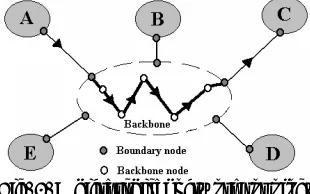
Another special case that we can apply Eqs. (21-24) to a general network topology is the case that we can express the network topology in a hierarchical manner as you can see in Fig. 3. In this figure, the gray areas represent users’ subnetworks and the dashed area represents the network backbone. If the network congestion occurs in the backbone, those users that are in a subnetwork and traverse the same route in the backbone, have the same
λ
i,nparameters that represent the congestion level in the user’s traffic route.
Fig. 3. A hierarchical network topology
In the general case, solving Eq. (19) with respect to ‘k’ is very difficult, but as it is shown in Section 4, some iterative methods can be used for converging towards the exact solution of ‘k’.
As you will see in the next section, we have used an iterative method by which we can converge towards the exact ‘k’ parameter in a general network topology.
Although we may lose the loss-free property in some occasions because of inaccurate estimation of ‘k’ in the initial steps of the iterative method, it is shown by simulation that the proposed iterative method has no loss with respect to Kelly’s method, at least in the simulated scenarios. The stability and convergence property of the revised method cannot be proved by Eq. (20), therefore these properties must be proved using theorem 2.
Theorem 2: Consider the following continuous-time system:
∑
∈
=
r
R j j r
r r
r(t) k (X) (ω -x (t) µ (t))
x dt
d
(25)
where
∑
∈
=
s
R j : s s j
j(t) ( x (t))
µ p
We further assume that:
R r 0 (X)
kr > ∀ ∈ (26)
Then the function:
∑ ∫
∑
∈ ∈
∆ ∑
∈
− =
J j
x
0 j
R
r r r
s R j
s: s (y)dy
x log ω ) X (
V p (27)
is a Lyapunov function for the above system and the vector X maximizing V(X)is a stable point of the system, to which all trajectories converge [2].
Proof: See the Appendix.
4. SIMULATION
Fig. 4. The first topology with 3 users and 2 links
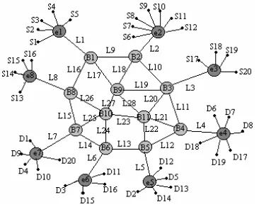
Fig. 5. The second topology with 20 users and 28 links
As we have used the macroscopic fluid-flow traffic model [1] for our purpose and considering the behavior of network queues and packet-level processing of network traffic (microscopic model) are not important for us, the MATLAB® package seems to be a good candidate for performing simulations. With
this package, we have simulated the networks and compared the proposed method with that of Kelly. The strategy for finding ‘k’ is based on the following iteration:
R i , ]} ω λ
. x ). 1 [( λ . tanh{x ε k
ki,n+1= i,n − i,n i,n − −ρi i,n-1 i,n-1+ρi i ∀ ∈ (28)
In which, ε>0 is some small constant.
The idea behind iteration (28) is that each user tries to follow the exact solution to (19) with one sampling delay and based on the most recent traffic information.
If ki,n in relation (28) converges for every ‘i’, the resulting k*i is the exact solution to Eq. (19) for every ‘i’.
The important point which must be mentioned here is that, each user for computing his or her corresponding
k
i,n, parameter, only needs theλ
i,nwhich might be available to him from the network by designing an appropriate network layer protocol. This results in distributed solution [13] fork
i,n. The simulation consists of two parts:a) Lack of loss in rate allocation of the Kelly method
In this part, the ‘k’ parameter for the Kelly method and the initial ‘k’ in the proposed method are selected small enough for the users. So, there is not any loss event in the network.
For topology of Fig.4, we have selected ‘k’ of the Kelly method and the initial ‘k’ of the proposed method in the iteration (28) to be 0.0009.
The normalized link capacity for all links is selected to be 30. We have also used R
r , 01 . 0
r = ∀ ∈
ρ and ε=0.01 in relation (28).
We have selected σ=1 and γ=600 in equation (10).
The users’ utility functions are in logarithmic form with the following parameters:
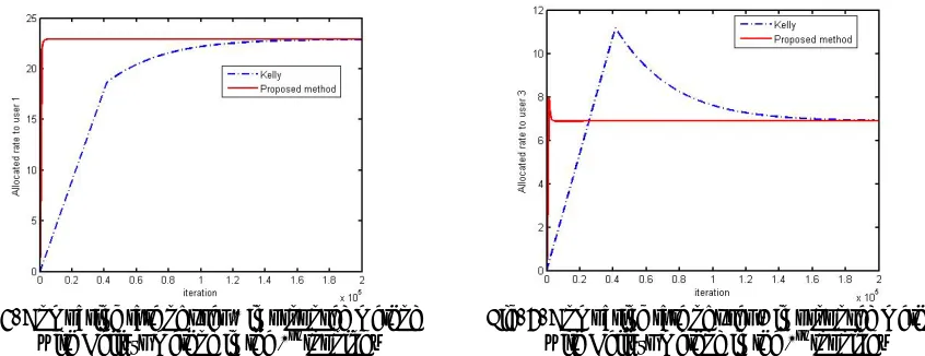
It can be verified in Figs. 6-7 that the rate allocated to users 2 and 3 have a higher convergence rate in the proposed method.
Fig. 6. Comparing rate of user 1 in proposed method
with Kelly’s method in the 1st topology Fig. 7. Comparing rate of user 3 in proposed method with Kelly’s method in the 1st topology
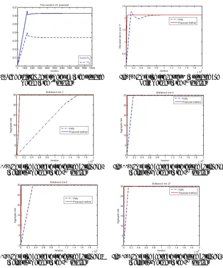
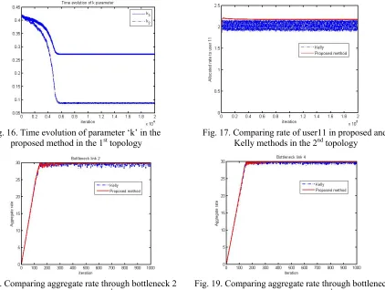
The time evolution of ‘k’ parameters in the proposed method for typical users 2 and 3 are depicted in Fig. 8.
The second network topology is depicted in Fig. 5 in which 20 users, denoted: by ‘S’ are traversing a network which consists of 28 links and each user’s destination denoted by ‘D’ letter. The links that are traversed by each user traffic are shown below:
Table 1. The route traversed by each user traffic in topology 2
User 1: L1-L17-L27-L25-L7 User 11: L2-L18-L27-L24-L6
User 2: L1-L17-L27-L23-L22-L5 User 12: L2-L10-L20-L22-L5
User 3: L1-L17-L27-L24-L6 User 13: L8-L26-L24-L13-L5
User 4: L1-L16-L15-L7 User 14: L8-L26-L24-L13-L5
User 5: L1-L17-L27-L23-L22-L5 User 15: L8-L26-L24-L6
User 6: L2-L10-L11-L4 User 16: L8-L15-L14-L6
User 7: L2-L10-L11-L4 User 17: L3-L20-L21-L4
User 8: L2-L10-L11-L4 User 18: L3-L20-L21-L4
User 9: L2-L18-L27-L25-L7 User 19: L3-L11-L4
User 10: L2-L18-L27-L25-L7 User 20: L3-L19-L27-L25-L7
For topology of Fig. 5 we have selected ‘k’ of the Kelly method and the initial ‘k’ of the proposed method in the iteration (28) to be 0.001.
The normalized link capacity for all links is selected to be 30. We also have used ρr =0.01 ,∀r∈Rand
ε=0.01 in relation (28).
We have selected σ=1 and γ=600 in Eq. (10). The users’ utility functions are in logarithmic form with the following parameters:
Table 2. User utility function parameters for topology 2
ω(1) = 0.5 ω(5) = 0.4 ω(9) = 0.25 ω(13) = 0.3 ω(17) = 0.2
ω(2) = 0.5 ω(6) = 0.7 ω(10) = 0.3 ω(14) = 0.2 ω(18) = 0.25
ω(3) = 0.3 ω(7) = 0.3 ω(11) = 0.2 ω(15) = 0.25 ω(19) = 0.3
ω(4) = 0.3 ω(8) = 0.25 ω(12) = 0.25 ω(16) = 0.3 ω(20) = 0.2 In Fig. 9, the rate allocated to the typical user 11 has been compared between the proposed method and Kelly method. It can be verified that the proposed algorithm has a higher convergence rate.
In Figs.10-13, the aggregate rates through bottleneck links "2","4","8" and "27" have been compared and it can be concluded that the proposed method is faster in convergence rate.
Fig. 8. Time evolution of parameter ‘k’ in the proposed
method in the 1st topology Fig. 9. Comparing rate of user11 in proposed and Kelly methods in the 2nd topology
Fig. 10. Comparing aggregate rate through bottleneck 2
in different methods in the 2nd topology Fig. 11. Comparing aggregate rate through bottleneck 4 in different methods in the 2nd topology
Fig. 12. Comparing aggregate rate through bottleneck 8
in different methods in the 2nd topology Fig. 13. Comparing aggregate rate through bottleneck 27 in different methods in the 2nd topology
b) Loss in rate allocation of the Kelly method
In this part, the parameter ‘k’ in the Kelly method is higher than part (a) and loss occurs in the network.
For the topology of Fig. 4 the ‘k’ parameter of the Kelly method and the initial ‘k’ of iteration (28) are selected to be 0.4. Other parameters are the same as part (a).
In Fig.15 the aggregate rate through typical bottleneck link "2" are compared between the Kelly and the proposed methods.
The number of loss events (when the aggregate rate through a link exceeds its capacity) in the Kelly and the proposed method are 50 and 0 respectively.
Fig. 14. Time evolution of two typical ‘k’ parameters in
the proposed method in the 2nd topology Fig. 15. Comparing aggregate rate through bottleneck 2 in different methods in the 1st topology
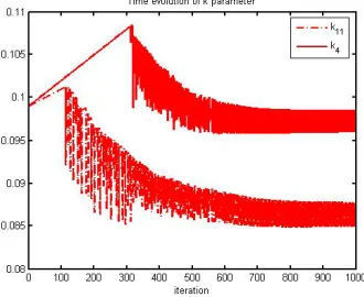
For the topology of Fig. 5 the ‘k’ parameter of the Kelly method and the initial ‘k’ of iteration (28) are selected to be 0.095. Other parameters are the same as part (a).
In Fig. 17, the rate allocated to the typical user 11 has been compared between the proposed and Kelly methods.
In Figs. 18-21 the aggregate rates through bottleneck links "2","4","8" and "27" have been compared between the Kelly and the proposed methods.
The time evolution of ‘k’ parameters in the proposed method for typical users 4 and 11 are depicted in Fig. 22.
The number of loss events in the Kelly and the proposed method are 1092 and 0 respectively.
It must be mentioned that the correct selection of the simulation parameters is of crucial importance in having a realistic simulation scenario.
For example, the incorrect selection of γ and σ parameters of the penalty function as it can be checked in Fig.1, can lead us to an incorrect estimation of ideal link penalty function.
Fig. 16. Time evolution of parameter ‘k’ in the
proposed method in the 1st topology Fig. 17. Comparing rate of user11 in proposed and Kelly methods in the 2nd topology
Fig. 18. Comparing aggregate rate through bottleneck 2
Fig. 20. Comparing aggregate rate through bottleneck 8
in different methods in the 2nd topology Fig. 21. Comparing aggregate rate through bottleneck 27 in different methods in the 2nd topology
Fig. 22. Time evolution of two typical ‘k’ parameters in the proposed method in the 2nd topology
5. CONCLUSION
One of the deficiencies of the Kelly’s method in [2] is the lack of presentation of a way by which each user can compute its ‘k’ parameter in a distributed way so that he (she) can ensure the loss-free property in his (her) allocated rate.
In this work, we have presented an algorithm by which users can change their ‘k’ parameter and the loss-free property of the allocated rate is guaranteed in a number of network topologies. We have investigated three different scenarios of communication networks including a simple one link-one user
scenario, one link-multi user case and general multi user-multi link case. For a general network topology, finding an analytic and distributed solution for equation (19) is very difficult, thus we have tried to find an approximate and distributed solution for ‘k’ parameter. For this purpose we have used penalty function (10) and iterative method (28) and have shown by simulation that, the proposed method has a higher convergence rate and no loss with respect to the Kelly method.
One shortcoming of this distributed solution is that the proposed rate allocation algorithm may not be loss-free in general, but the important point about the approximate method in (28) is its distributed structure, i.e., each user can choose its ‘k’ parameter intelligently with only the help of the congestion parameters λi,nandλi,n-1 that are fed back to him from the network.
NOMENCLATURE
A routing matrix
cj link ‘j’ capacity
C links capacity vector
kr gain parameter for user ‘r’
(.)
j
p
link ‘j’ penalty functionR set of network users
T time (iteration)
ur(.) user ‘r’ utility function U vector of user utility functions
V(.) lyapunov function
xr rate (throughput) allocated to user ‘r’ X users’ allocated rate vector
Greek letters
ε small positive gain parameter
γ
penalty function parameteri
λ aggregate penalty of user i’s route
(.)
µ
j link ‘j’ penalty functionωr user ‘r’ utility function parameter
Ω
user’s utility function parameter vectorγ
penalty function parameterρ
gain parameter in our algorithmσ penalty function parameter
REFERENCES
1. Jacobson, V. (1988). Congestion avoidance and control. Comput. Commun. Rev., 18(4), 314-329.
2. Kelly, F., P., Maulloo, A. K. & Tan, D. K. H. (1998). Rate control for communication networks: shadow prices, proportional fairness and stability. J. Oper. Res. Soc., 49(3), 237-252.
3. Sheikholeslam, F., Tahani, V. & Zangeneh, H. R. Z. (2000). Periodic solutions of nonlinear equations based on extended stability theorems of nonlinear systems. Iranian Journal of Science & Technology, 24(1), 111-117 4. Tahani, V. & Sheikholeslam, F. (1999). Total stability of fuzzy feedback control systems. Iranian Journal of
Science & Technology, 23(Jan), 7-34
5. Teshnelab, M. & Afyooni, D. (2004). An artificial intelligent system for traffic forecasting in virtual stations of highways Tehshnehlab. Iranian Journal of Science and Technology, Transaction B: Engineering, 28(3) B, 2004, pp 395-400
6. Shenker, S. (1995). Fundamental design issues for the future Internet. IEEE J Selected Areas Commun., 13(7), 1176-1188.
7. Kelly, F. P. (1997). Charging and rate control for elastic traffic. Eur. Trans. Telecommun., 8, 33-37.
8. Mo, J. & Walrand, J. (2000). Fair end-to-end window-based congestion control. IEEE/ACM Transactions on Networking, 8(5), 556-567.
9. Massoulié, L. & Roberts, J. (1999). Bandwidth sharing: objectives and algorithms. Proc. IEEE INFOCOM, 3, New York, 1395-1403.
10. Bertsekas, D. & Gallager, R. (1987). Data networks. Prentice Hall, Englewood Cliffs, NJ.
11. Kunniyur, S. & Srikant, R. (2000). End-to-end congestion control schemes: utility functions, random losses and ECN marks. IEEE INFOCOM 2000-Tel Avive, Israel.
12. La, R. J. & Anantharam, V. (2002). Utility-based rate control in the internet for elastic traffic. IEEE Trans. On Networking, 10(2), 272-286.
APPENDIX
S. M. Proof of theorem 2:
We will follow the lines of proof, which is presented in [1] with some modifications.
The assumptions on ωr >0, r∈R and pj, j∈J ensure that V(X) is strictly concave on X≥0 with an
interior maximum; the maximizing value of X is thus unique. Observe that:
∑
∑
∈ ∈
− = ∂
∂
r s
R
j j s:j R s r
r
r
) x ( x
ω ) X ( V
x p (a)
Setting these derivatives to zero identifies the maximum. Furthermore, we have:
∑
∑
∑
∑
∈ ∈ ∈
∈
⎟ ⎟ ⎠ ⎞ ⎜
⎜ ⎝ ⎛
⎟ ⎟ ⎠ ⎞ ⎜
⎜ ⎝ ⎛ −
⋅ ⋅ =
∂ ∂ =
R r
2
R s: R s
r r r r
r R
r r
r s
x .
x ω x
1 (X) k
t) ( x dt
d . x ))
t ( X ( V dt
d
j j j
p ϑ
(b)
As kr(X) is a positive parameter with a positive limit as t goes to infinity, it can be easily verified that
V(X(t)) is strictly increasing with ‘t’, unless X(t)=X*, the unique Xmaximizing V(X(t)) which is the same
solution as Eq. (4) displays. Thus the function V(X(t)) is a Lyapunov function for the system.