S. Descombes, B. Dussoubs, S. Faure, L. Gouarin, V. Louvet, M. Massot, V. Miele, Editors
A 3D FINITE VOLUME SCHEME FOR THE SIMULATION OF EDGE PLASMA
IN TOKAMAKS
∗M. Bilanceri
1, L. Combe
1, H. Guillard
1, B. Nkonga
1et A. Sangam
1R´esum´e. Une m´ethode de volumes finis en coordonn´ees cylindriques pour la simulation de la r´egion du bord dans les tokamaks est propos´e. Contrairement aux m´ethodes classiques, qui sont bas´es sur la projection des ´equations en coordonn´ees curvilignes, une nouvelle m´ethode est propos´ee ici. Cette technique est bas´ee sur la discr´etisation de la forme vectorielle des ´equations et ensuite sur la projection sur les vecteurs de base du syst´eme curviligne associ´e `a chaque volume de contrˆole. La M´ethodologie propos´ee a ´et´e valid´ee sur plusieurs cas-tests simples et appliqu´e sur une simulation 3D d’un mod`ele MHD r´eduit.
Abstract. A finite volume method in cylindrical coordinates for the simulation of the edge region in tokamaks is proposed. In contrast to standard methods, which require the projected form of the equations in curvilinear coordinates, a new method is proposed. This technique is based on the dis-cretization on the vector form of the equations and then on the projection on the basis of the curvilinear system associated to each control volume. The proposed methodology has been validated on several simple test cases and applied on a 3D simulation of a reduced MHD model.
Introduction
Due to the rarefaction of fossil energies as well as their adverse effects in term of environmental issues, the research of alternative energy sources is a major issue in the coming years. Among others, magnetically confined, controlled thermonuclear fusion is a promising possibility that leads to the construction of experimental reactors called Tokamaks (like ITER in Cadarache) to explore the feasibility of this concept. Many technical and conceptual difficulties have however to be overcome before the actual use of fusion energy. The recourse of numerical simulation methods will play a decisive role in this context allowing a better understanding of the physical phenomena and improvement in the design and performance of the machines. The objective of this work is to develop numerical models for the simulations of edge plasma in tokamak reactors in the framework of fluid modeling. From a purely numerical standpoint, the simulations of existing (TORE-SUPRA, JET, ...) and future (WEST, ITER, DEMO, ...) tokamak devices must now be able to consider realistic complex geometries. Due to the requirement to obtain quantitative prediction that can be used in the actual design of the machines, the use of simple finite difference approximations associated to analytic definition of the magnetic field lines is no more appropriate and more sophisticated numerical tools have to be developed [4]. In this work, we have chosen to concentrate on a finite volume approach that has potentially the capability to incorporate high order schemes with desired regularity of shape functions. Finite volume methods are specialized techniques to approximate systems of conservation laws. However, since tokamaks are axisymmetric devices, the use of the
∗thanks to ANR ESPOIR which funds the work of M. Bilanceri and L. Combe
1Inria Sophia-Antipolis 2004 Route des Lucioles, BP 93, 06902 Sophia-Antipolis Cedex and Univ. Nice Sophia Antipolis, LJAD,
UMR 7351, 06100 Nice, France
c
EDP Sciences, SMAI 2013
Cartesian coordinate system is not the most appropriate to the geometry of the problem. Unfortunately, the application of FV methods to curvilinear systems of coordinate is problematic because the space variation of the metric coefficients introduces artificial source terms. However it can be shown that whatever the curvilinear system used, a strong conservation form of the equations exists at the level of vector variables. Note that this strong conservation form do not exist at the level of the scalar components of the vectors in the curvilinear system due to the aforementioned space dependence of the metric coefficients. Based on this result, we report in this work on the design of an original Finite Volume technique that uses an approximation of the vector form of the equation followed by a local projection on the curvilinear system. This paper is organized as follows : Section 1 gives the basis of our approach and explain how to deal with curvilinear system of coordinate in a general way. Section 2 details this approach for the specific case of the toroidal geometry of tokamaks and gives the geometric computations necessary to implement the method. Section 3 presents the final finite volume method. Finally, in the last section, we apply this technique to a reduced MHD model.
1.
The discretization-projection method
Let us consider a general hyperbolic conservation laws equation written in a coordinate free manner as
∂W
∂t +∇ ·F(W) = 0, whereWis the state variable andF(W) is its flux.
Let us also consider a curvilinear transformationφ:ξ7→x, whose determinant of Jacobian isJ. It is possible to show [1], that in this coordinate system, the above equation becomes:
∂W ∂t +
1 J
∂ ∂ξk
JF(W)·ek
= 0.
where ek are the contravariant basis vector associated to the transformation φ: ξ 7→ x. Let us consider the special case withW=V is a vector andF(W) =Tis a tensor. The hyperbolic equation turns into :
∂V ∂t +
1 J
∂ ∂ξk
JT·ek
= 0. (1)
The momentum equation in fluids dynamics is such a kind of equations.
Note that, sinceVis a vector, it has to be stored component by component on a given basis. The traditional approach consists in taking the scalar product of equation (1) by the covariant basis vectors ek and then to obtain scalar equations for the components of the vector fieldV. Finally these scalar equations are discretized. In the sequel, we will designate this method as the projection-discretization method. This approach has one important shortcoming : because the basis vectors are spatially dependent, they do not commute with the differential operators and therefore source terms appear in the equations [1, 5]. The expression of these source terms depends on the specific curvilinear system used and their approximation is not obvious if some properties as for instance angular momentum conservation are required.
We therefore advocate the use of the following procedure that we will be called the discretization-projection method. First we define an auxiliary reference system associated to the ith-cell. This auxiliary system is coincident with the curvilinear reference system in center of mass of the cell. The second step is to consider the integral formulation of (1), that is :
∂ ∂t
Z
V
VdV+ I
S
T·ndS= 0 (2)
Sec. 2. Finally the discretized version of (2) is projected on the auxiliary reference system by simply taking the dot product between the discretized equation and the auxiliary basis vectors.
Note that in the standard projection-discretization approach first the continuous equation is projected and the resulting scalar equations are discretized while in our discretization-projection method first we discretized a vector equation and then we project the results. This procedure is quite simple and it allows for a general (and implicit) discretization of the curvature terms.
2.
Toroidal geometry and mesh generation
Since, the geometry of a tokamak is axisymmetric, it can be considered as the revolution of a plane, the poloidal plane, about an axis. The description of this kind of geometries, as well as the development of numerical methods, is much easier if, instead of the standard Cartesian system of coordinates, we use a cylindrical coordinate system.
2.1.
System of coordinates
Let us consider a standard Cartesian system of coordinates (x, y, z) where thez-axis is coincident with the axis of revolution of the poloidal plane. The coordinates R, ϕ, Z are related to the standard Cartesian coordinates as
x=Rcosϕ
y=Rsinϕ
z=Z
or
R=px2+y2
ϕ=
0 ifR= 0
arccos (x/R) ify≥0 2π−arccos (x/R) ify <0
z=Z
(3)
Given the position vectorx= (x, y, z), we will noteeR,eϕ,eZ the covariant basis associated to the transforma-tion (3), that is
eR= ∂x ∂r =
∂x ∂ri+
∂y ∂rj+
∂z ∂rk eϕ=
∂x ∂ϕ =
∂x ∂ϕi+
∂y ∂ϕj+
∂z ∂ϕk eZ =
∂x ∂z =
∂x ∂zi+
∂y ∂zj+
∂z ∂zk
(4)
The Jacobian of the transformation is defined by
J =eR·(eϕ×eZ) =R (5)
The basis vector in (4) are not normalized and, thus, we will use the notation
˜
eR=eR/|eR|, ˜eϕ=eϕ/|eϕ|,˜eZ =eZ/|eZ| (6) for unit vectors of the basis.
2.2.
Common operations using the cylindrical system of coordinates
In the following we will consider some common mathematical operation that are needed in the development of the numerical scheme. In particular the standard Cartesian formulation and its equivalent formulation in the cylindrical coordinate system are considered. The first operation is the integration of a scalar function f over a volumeV :
Z
V
fdV= Z
V(x,y,z)
f(x, y, z)dxdydz= Z
V(R,ϕ,Z)
Note that using this approach the measure of a control volume, which will be denoted byV3Dis defined by:
V3D=. Z
V
dV = Z
V(x,y,z)
dxdydz= Z
V(R,ϕ,Z)
RdRdϕdZ (8)
Also, the average value of a function over a control volume,fave, is simply defined by the following relation:
fave= Z
V
fdV
Z
V
dV
= Z
V
fdV
V3D (9)
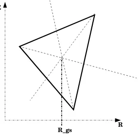
Let us consider a surfaceS in the (R, Z)-plane; for this surface it possible to define two different measures, the 2Dmeasure, S2(R,ZD ), and the “toroidal” one,S(R,Z), which are defined by:
S2(R,ZD )=. Z
S(R,Z)
dRdZ S(R,Z)=. Z
S(R,Z)
RdRdZ=S2(R,ZD )RgS (10)
whereRgS is theR-coordinate of the center of mass of the surfaceS.
R Z
R_gs
Figure 1. Definition of the center of gravity of a surface in the poloidal plane
-A kind of control volume which is particularly important for our case is the one which is obtained by the rotation of a surfaceS in the (R, Z)-plane around theZ-axis. Let defineϕ1 andϕ2as the starting and ending
angles of revolution; the measure of this control volume can be easily calculated as follows:
V3D=. Z
V
dV= Z ϕ2
ϕ1
Z
S(R,Z)
RdRdZdϕ= ∆ϕS(R,Z) (11)
where ∆ϕ=ϕ2−ϕ1. Even for a segmentI in the (R, Z)-plane it is possible to define two different measures,
a 1D measure,I1(R,ZD )and a toroidal one,I(R,Z), defined as follows:
I1(R,ZD )=. Z
l
dl I(R,Z)=. Z
l
R(l)dl=I1(R,ZD )RgI (12)
anglesϕ1 andϕ2 of a segmentI in the (R, Z) plane . The measure of this surface,S(l,ϕ), can be computed as
follow:
S(l,ϕ)=.
Z
S
dS = Z ϕ2
ϕ1
Z
l
R(l)dldϕ= ∆ϕI(R,Z) (13)
Finally, let us consider a vectorVwhich is independent onϕand whose non zero components are always in the (R, Z)-plane, that is:
V=VR(R, Z)˜eR+Vz(R, Z)˜eZ (14) In the development of the numerical scheme it will be required to integrate this kind of vectors over a poloidal surface Spol. To compute this integral it is useful to consider an auxiliary Cartesian reference system defined as follows:
i=˜eR(ϕ), j=˜eϕ(ϕ), k=˜eZ, ϕ=
ϕ2+ϕ1
2 (15)
Using this auxiliary reference system the expression of the vectorV becomes:
V= cos ˜ϕVR(R, Z)i+ sin ˜ϕVR(R, Z)j+VZ(R, Z)k, ϕ˜=ϕ−ϕ (16) And, thus the expression of the integral ofVoverSpol becomes:
Z
Spol
VdS= Z ∆2ϕ
−∆ϕ 2
Z
l
(cos ˜ϕ VR(R, Z)i+ sin ˜ϕ VR(R, Z)j+VZ(R, Z)k)Rdldϕ˜=
Z
l
VR(R, Z)i
sin
∆ϕ 2
−sin
−∆ϕ
2
Rdl
−
Z
l
VR(R, Z)j
cos ∆ϕ
2
−cos
−∆ϕ
2
Rdl
+ Z
l
∆ϕ VZ(R, Z)kRdl= Z
l
2 sin ∆ϕ
2
VR(R, Z)i+ ∆ϕ VZ(R, Z)k
Rdl
= Z
l
2 sin ∆ϕ
2
VR(R, Z)˜eR(ϕ) + ∆ϕ VZ(R, Z)˜eZ
Rdl (17)
where the last equivalent follows from (15) and the fact that ˜eR is independent onR and Z. Finally in the special case whereVR andVZ are constants the integration reduces to:
Z
Spol
VdS= 2
∆ϕsin ∆ϕ
2
VR˜eR(ϕ) +VZ˜eZ
S(l,ϕ) (18)
One important application of (18) is the computation of the (average) normal vector to a surfaceSpol. Indeed, in this case we can replace Vwith nI, the normal to the segment from whichSpol is generated. SinceI is a segment, nI is a constant in the (R, Z) plane. Thus, by integrating nI over the surface Spol it is possible to define the (average) normalntoSpol which, from (18) is
nS(l,ϕ)=
2
∆ϕsin ∆ϕ
2
nI,R˜eR(ϕ) + nI,Z˜eZ
S(l,ϕ) (19)
2.3.
Integration of a vector polynomial function
In this subsection we will compute the integration of a vector polynomial function using the cylindrical system of coordinates. First let us recall the following identities:
∂˜eR ∂ϕ =˜eϕ,
∂˜eϕ
(˜e
R(α)−˜eR(−α) = 2 sin (α)˜eϕ(0) ˜
eϕ(α)−˜eϕ(−α) =−2 sin (α)˜eR(0) (˜e
R(α) +˜eR(−α) = 2 cos (α)˜eR(0) ˜
eϕ(α)−˜eϕ(−α) = 2 cos (α)˜eϕ(0)
(21)
The integral that we want to compute is of the following form:
Z ∆2ϕ
−∆ϕ 2
f(ϕ)dϕ (22)
assuming that f(ϕ) is a polynomial function in ϕ (and thus f(ϕ) ∈ C∞). Note that the form (22) is quite general. Indeedf can be the results of an integration in the (R, Z)-plane such asf(ϕ) =R(R,Z)g(R, ϕ, Z)dRdZ. First, let us focus on the following special case:
Z ∆2ϕ
−∆ϕ 2
˜
eRf(ϕ)dϕ (23)
By using (20)-(21) and by repeatedly integrating by part it is possible to obtain
Z ∆2ϕ
−∆ϕ 2
˜
eRf(ϕ)dϕ=− Z ∆2ϕ
−∆ϕ 2
∂˜eϕ
∂ϕf(ϕ)dϕ=−˜eϕf|
∆ϕ 2
−∆ϕ 2
+ Z ∆2ϕ
−∆ϕ 2
˜
eϕf0(ϕ)dϕ=
−˜eϕf|∆2ϕ
−∆ϕ 2
+ Z ∆2ϕ
−∆ϕ 2
∂˜eR ∂ϕf
0(ϕ)dϕ= −˜eϕf|∆2ϕ
−∆ϕ 2
+˜eRf0|∆2ϕ
−∆ϕ 2
−
Z ∆2ϕ
−∆ϕ 2
˜
eRf00(ϕ)dϕ=...
−˜eϕ(f−f00+f0000− · · ·)|
∆ϕ 2
−∆2ϕ+˜eR(f
0−f000+f00000− · · ·)|∆2ϕ
−∆2ϕ (24)
where g|βαmeans
g|βα=. g(β)−g(α) (25)
Let us break down any product ˜e?g|βα where? can beR orϕin the following way :
˜ e?g|
β
α=g∆˜e?+˜e?∆g (26)
where
k= k(β) +k(α)
2 , ∆k=k(β)−k(α) (27)
Using (26) and (21) it is possible to recast (24) as follows:
˜ eR(0)
2 sin ∆ϕ 2 f+ cos ∆ϕ 2
∆f0−2 sin ∆ϕ 2 f00 − cos ∆ϕ 2
∆f000−2 sin ∆ϕ 2 f0000 +· · · +
˜eϕ(0)
2 sin ∆ϕ
2
f0−cos ∆ϕ 2 ∆f − 2 sin ∆ϕ 2
f000−cos ∆ϕ
2
∆f00
+· · ·
Note that the general term2 sin∆2ϕfk+1−cos∆2ϕ∆fkis at least a second-order term as function of ∆ϕ
lim
∆ϕ→0
1 ∆ϕ
2 sin
∆ϕ
2
fk+1−cos ∆ϕ
2
∆fk
=
lim
∆ϕ→0
2
∆ϕsin ∆ϕ
2
fk+1−cos ∆ϕ
2 ∆fk
∆ϕ
= lim
∆ϕ→0
fk+1−∆f
k
∆ϕ
= 0
(29)
Indeed it is of the order ∆ϕ2. If a first-order or a second-order scheme is considered, this terms can be safely neglected in the integration process but for high-order methods (more than second-order) they should be taken into account. Using the same approach it should be straightforward to compute the integral of
Z ∆2ϕ
−∆2ϕ ˜
eϕf(ϕ)dϕ (30)
Finally we can compute the integral of a general vector polynomial function by simply using the identity
Z ∆2ϕ
−∆ϕ 2
f(ϕ)dϕ= Z ∆2ϕ
−∆ϕ 2
˜eRfR(ϕ)dϕ+ Z ∆2ϕ
−∆ϕ 2
˜
eϕfϕ(ϕ)dϕ+ Z ∆2ϕ
−∆ϕ 2
˜
eZfZ(ϕ)dϕ (31)
2.4.
Mesh generation
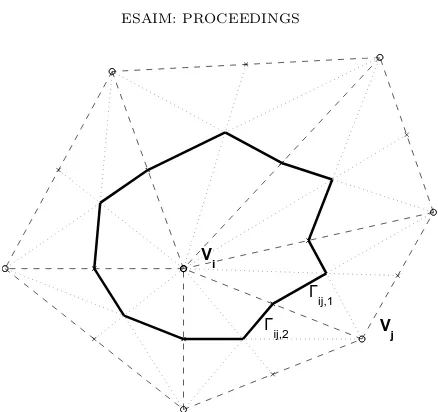
The generations of the mesh, which we will use in our code, exploit the features of tokamaks geometries. Since the geometry of the poloidal plane could be arbitrary complex, as a first step an unstructured 2D dual mesh is generated. First, the considered computational domain (the poloidal plane), is divided intoNttriangles. LetTj denotes thejth-triangle; theithfinite-volume cellVi, associated with theith-vertex is given by
Vi= [
j Vi(j)
where the union is extended to all the triangles sharing theith-vertex andV(j)
i represents the subset ofTjwhich is defined by further dividing Tj into six sub-triangles by means of its medians and subsequently considering those two sub-triangles which share theith-vertex (see figure 2). As shown in Fig. 2, the interface between the ith-cell and the jth-one is composed by two segments, Γ
ij,1 and Γij,2. Once a 2D mesh is generated the 3D
mesh is generated by the revolution of the poloidal mesh about the axis of revolution. In practice the interval [0,2π] is divided intoNplansegments defined by the points ϕ1, ϕ2,· · ·, ϕNplan
. For each 2Dcontrol volumeVi we obtainNplan3Dcontrol volumesVi3Dwhich are obtained by the rotation ofVi between the anglesϕk, ϕk+1
(A similar argument holds true even for the triangles of the 2D mesh). Note that the boundary of the generic control volumeV3D
i can be divided into two kinds of surfaces, the poloidal surfacesSpoland the toroidal ones,
Stor. The poloidal surfaces are obtained by the revolution of the segments Γ
ij,1 and Γij,2of the poloidal mesh.
The toroidal surfaces are always two and are the images of the revolved 2D control volumeVi.
3.
Numerical discretization
In this section we will consider the discretization of the isothermal Euler model:
∂n
∂t +∇ ·nu= 0 ∂nu
∂t +∇ ·(nu⊗u) +∇p=0
V i
V j Γij,1 Γij,2
Figure 2. Generation of the dual Mesh.
wherec2 is the square of the (constant) sound speed,
A Finite-Volume formulation is considered to discretize the convective part of system (32) and, thus, it is convenient to recast system (32) in the following integral form
∂ ∂t
Z
V
ndV+ I
S
nu·ndS = 0 (33a)
∂ ∂t
Z
V
nudV+ I
S
(nu⊗u)·ndS+ I
S
pndS=0 (33b)
which, by using a standard finite-volume discretization over theithcontrol volume becomes
V3D i
∂ ∂tni+
X
j Z
Sij
fn(Wi, Wj,nij)dS = 0 (34a)
V3D i
∂ ∂tniui+
X
j Z
Sij
fu(Wi, Wj,nij)dS=0 (34b)
where the summation overjis extended to all the neighbors of the control volume andWi= (ni, nui) T
. Note in particular that since our 3Dcontrol volume is obtained by the revolution of a 2D surface we can distinguish two different kinds of surfaces, the poloidal and the toroidal ones. Thus, in the following it will be shown that it is useful to split the summation in system (34) as
V3D i
∂ ∂tni+
X
j∈Spol
Z
Sij
fn(Wi, Wj,nij)dS+ X
j∈Stor
Z
Sij
fn(Wi, Wjnij)dS = 0 (35a)
V3D i
∂ ∂tniui+
X
j∈Spol
Z
Sij
fu(Wi, Wj,nij)dS+ X
j∈Stor
Z
Sij
scheme [2]. Once a numerical flux function is defined, system (35) can be recast as
V3D i
∂ ∂t
ni
nui !
+ X
j∈Spol
Z
Sij
F(Wi, Wj,nij)dS+ X
j∈Stor
Z
Sij
F(Wi, Wj,nij)dS=0 (36)
The last step to completely define the spatial discretization of the convective fluxes is to describe the strategy employed to compute the surfaces integrals in (36). Since we want to exploit the curvilinear coordinate system associated to the toroidal geometry, the flux function will be expressed in the cylindrical coordinate system. Considering the definitions and properties demonstrated in Sec. 2.3 the computation of the surface integrals should be straightforward. In particular, if the flux function Fij is considered constant, the result of the integration over a poloidal surface and toroidal surface is given by
Z
Spol
F(Wi, Wj,nij)dS=S(l,ϕ)
Fn
2 ∆ϕsin
∆ϕ 2
FuReR(i) +Fuϕeϕ(i)
+FuZeZ(i)
(37a)
Z
Stor
F(Wi, Wj,nij)dS=S(R,Z)
Fn
FuReR(i) +Fuϕeϕ(i) +FuZeZ(i)
!
(37b)
where eR(i),eϕ(i),eZ(i) are the basis vectors associated to the ith-control volume. Note however that the proposed methodology is not restricted to constant flux function. Indeed by using the expressions in Sec. 2.3 it is possible to exactly integrated any polynomial function and, thus, it is possible to increase the order of the method. By using (37b) into (36) the resulting semi-discrete formulation is
Vi3D ∂ ∂t
ni
nui !
+ X
j∈Spol Sij(l,ϕ)
Fij,n
Fij,uR∆2ϕsin∆2ϕ
Fij,uϕ
2 ∆ϕsin
∆ϕ 2 Fij,uZ + X
j∈Stor Sij(R,Z)
Fij,n Fij,uR
Fij,uϕ
Fij,uZ
=0 (38)
3.1.
Second-order extension
To achieve the second-order extension in space a MUSCL-like technique as been employed [3]. First, a gradient is associated to each control volume, then at each interfacesS a reconstructed state is computed as
Wij =Wi+∇Wi·(sij−gi) Wji=Wj+∇Wj·(sij−gj) (39) where gi and gj are the centers of mass of the control volumes andsij is the midpoint of the segment joining gi andgj (which is on the surface by construction). Finally, the flux function is computed as a function of the reconstructed states, that is Fij = F(Wij, Wij,nij) instead of the first order method Fij =F(Wi, Wj,nij). To compute the gradient ∇Wi first the compute a non-limited gradient by exploiting the features of our mesh which is unstructured in the poloidal plane (R, z) and structured in the toroidal direction. As a consequence, the gradient in the toroidal direction is computed using a 1D centered approximation
(∇Wi)ϕ= 1 ri
Win−Wip ϕin−ϕip
(40)
is
(∇Wi)(R,Z)= P
jS (R,Z) Tj ∇Wi|Tj
P jS
(R,Z) Tj
(41)
where the summation is extended to all the triangular elements to which the ith node belongs, S(R,Z) Tj is the
surface in the (R, Z) of the triangle and ∇Wi|Tj is the gradient restricted to the triangleTj computed using
a standard P1 finite-element approximation. Finally the gradient considered in (39) is obtained by applying a Minmod like limiter to the previous computed non-limited gradient.
3.2.
Discretization of the diffusion term
In this section we consider a parabolic system of the following form
∂n
∂t =∇ ·(µnD∇n)
∂nuk
∂t =∇ · µuD∇ nukb
with (42)
The diffusion terms in (42) can be recast as surface integrals as
Z
V
∇ ·(µnD∇n)dV= Z
S
µn(D∇n)ndS (43)
with a similar expression for the momentum equation. Since in general in Finite-Volume methods the solution is only required to be piecewise continuous, it is necessary to define a gradient on the surfacesS. In this work we chose to use the following definition of the gradient
Z
Sij∩Tk
µn(D∇n)nijdS = Z
Sij∩Tk
µn(D∇n|Tk)nijdS (44)
whereSij∩Tkis the intersection between the surfaceSijand the triangleTkand∇n|Tkis the gradient computed
using a standard P1 finite element approximation, as in the previous subsection.
3.3.
Time advancing
For the time advancing we considered an explicit scheme. The first-order time advancing is obtained by simple using the Euler method, that is
ni nuk,i
n+1 =
ni nuk,i
n + ∆t
V3D i
RHSn (45)
where RHSn is the contribution of the convective and diffusive fluxes computed using the solution at time n. The second-order accuracy in time is obtained by using the a TVD RK2 [6] scheme, that is
ni nuk,i
n+1/2 =
ni nuk,i
n + ∆t
V3D i
RHSn (46a)
ni nuk,i
n+1 =
ni nuk,i
n + ∆t
2V3D i
4.
Numerical experiments
The numerical method described in the previous sections has been validated using several different test cases. A first test case is introduced in order to validate the discretization of the diffusion terms. Then an axisymmetric simulation using the JET geometry has been considered..
4.1.
Validation of the viscous terms
In order to validate the discretization of the viscous term two different test cases have been considered, a radial diffusion test case and a toroidal diffusion one. In both test-cases only isotropic diffusion is considered, that is we consider the following reduced system:
∂n
∂t =∇ ·(µn∇n)
∂nu
∂t =∇ · µu∇ nukb
(47)
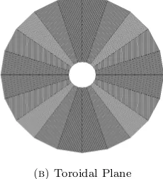
The computational domain restricted to the poloidal plane is a rectangle in the region 20≤R≤120, 0≤Z≤10 and it is meshed using 4696 points. In the computational domain 20 equidistant poloidal planes are used, as show in Fig. 3.
(a)Poloidal Plane
(b)Toroidal Plane
Figure 3. Mesh used for the diffusive test-cases.
4.1.1. Radial diffusion problem
In this test case we want to solve system (47) using the following boundary conditions
n|R
min= 1, n|Rmax= 10,
∂n ∂Z Z
min
= 0, ∂n ∂Z Z
max
anduis imposed equal to zero on all the boundaries. For this problem the analytic stationary solution is given byu= 0 and
n(R) =C1ln
R
Rmin
+C2 ⇒ n(R) =
9 ln 6ln
R
20
+ 1 (49)
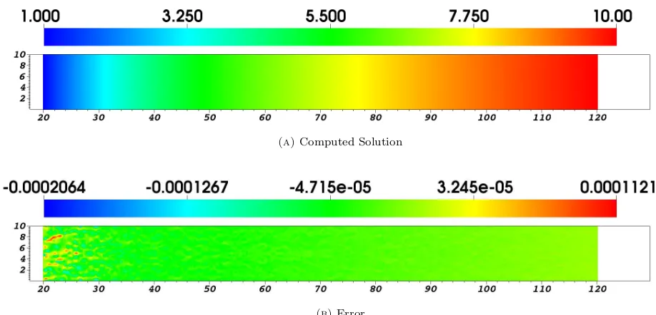
where the second expression is the one obtained using the boundary conditions in (48). We started our simulation with the analytic solution and we waited until the residual is below 10−7. In Fig. 4 the solution computed by
the numerical method and the error with the analytic one are shown. It is possible to see the good agreement between the reference and computed solution, thus validating the implementation of the diffusive terms in the poloidal plane.
(a)Computed Solution
(b)Error
Figure 4. Results for the radial diffusive test-case.
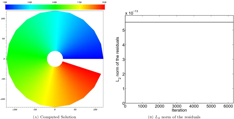
4.1.2. Toroidal diffusion problem
In this test case we consider a modified computational domain defined between the anglesϕmin≤ϕ≤ϕmax withϕmin= 0 andϕmax=1910π. The boundary conditions applied to (47) are the following
n|ϕ
min = 1, n|ϕmax = 10,
∂n ∂Z
Rmin
= 0, ∂n ∂Z
Rmax
= 0, ∂n ∂Z
Zmin
= 0, ∂n ∂Z
Zmax
= 0 (50)
anduis imposed equal to zero on all the boundaries. For this problem the analytic stationary solution is given byu= 0 and
n(ϕ) =C1+C2(ϕ−ϕmin) ⇒ n(ϕ) = 1 + 9
ϕ−ϕmin
ϕmax−ϕmin (51)
(a)Computed Solution
0 1000 2000 3000 4000 5000 6000
0 1 2 3 4 5
x 10−13
Iteration
L 2
norm of the residuals
(b)L2 norm of the residuals
Figure 5. Results for the toroidal diffusive test-case.
4.2.
A reduced MHD system
In this test-case we consider the simulation of the reduced MHD model:
∂n
∂t +∇ ·nu=∇ ·(µnD∇n) ∂nuk
∂t +∇ · nuku
+∇kp=∇ · µuD∇ nukb
+nu.Db Dt
with
u=ukb+
B× ∇Φ B2
Φ = ln n
n0
p=c2n, c= r
Te mi
(52)
where Te is the (constant) temperature of the electrons, mi is the ion mass, B is the magnetic field, b is the direction of the magnetic field. Φ is the electric potential evaluated thanks to the adiabatic assumption
Φ = ln n
n0
wheren0 is the average ofnover a magnetic surface. The quantity
B× ∇Φ
B2 is the electric drift
velocity. Finallyµn andµu are two diffusion coefficients andD is a diffusion tensor defined as
D=I−b⊗bT (53)
where I is the identity tensor. Note that the physical meaning ofD is that the diffusion is highly anisotropic; in particular there is no diffusion in the direction parallel to the magnetic field. System (52) can be scaled using the following reference values
˜ x= x
Lref, n˜= n
nref, u˜k= uk
c , ˜t=t c Lref,
˜ Φ,= Φe
Te ˜ B= B
and, as consequence, we can derive the following adimensionalized quantities
˜
u= ˜ukb+ρ? ˜ B× ∇Φ˜
˜
B2 , ρ
?
= mic eB0Lref
, µn˜ = µn
Lrefc, µu˜ = µu Lrefc,
Note in particular the expression of the adimensionalized velocity; the adimensionalized factorρ?, which is the adimensionalized Larmor radius, multiplies the term associated to the drift velocity. Indeed this shows thatρ? is an indicator of the ratio between the parallel and drift components of the velocity. Given the results of section 2, the discretization of this model is straightforward. It is clear that the momentum equation for the parallel velocity uk is nothing but the projection of the vector momentum equation on the direction of the magnetic field. Therefore it is sufficient to project the momentum equation on the direction parallel to the magnetic field. Indeed, by definingbi the direction of the magnetic field in the control volume, it follows
u·bi=
uk,ibi+
Bi× ∇Φi B2
i
·bi=uk,i (54)
and, thus using the results of section 3, we obtain from (38)
V3D i
∂ ∂tni+
X
j∈Spol
Sij(l,ϕ)Fij,n+ X
j∈Stor
Sij(R,Z)Fij,n= 0 (55a)
V3D i
∂
∂tnuk.i+bi·
X
j∈Spol Sij(l,ϕ)
Fij,uR
2 ∆ϕsin
∆ϕ 2
Fij,uϕ∆2ϕsin∆2ϕ
Fij,uZ
+ X j∈Stor
Sij(R,Z)
Fij,uR
Fij,uϕ
Fij,uZ
= 0 (55b)
that provides a complete description of the numerical algorithm.
In the considered test case the magnetic geometry contains an X point and the 2D mesh is aligned on the field lines in the poloidal plane. Note however that our method do not require any specific arrangement for this case. The mesh of the poloidal plane consists of 3564 points while 50 poloidal planes are considered. As for the diffusion coefficients,µn andµu, we have used the valuesµn= 1m2/s andµu= 0.1m2/s. Finally the value of ρ? is set equal to 3·10−4 resulting in a drift velocity of the order of some percents of the speed of sound, typically the ones experimentally found in the SOL. Considering the boundary conditions, on the inner surface a constant gradient of density, equal to −1, and uk = 0.5cs are imposed. On the outer surface two limiters are present where Bohm boundary conditions are imposed. Bohm boundary conditions require that the flow goes out of the computational domain with a speed at least equal to the speed of sound. On the remaining of the outer surface standard slip conditions are imposed. Note that using this set of boundary conditions and a constant initial condition the resulting simulations are axisymmetric.
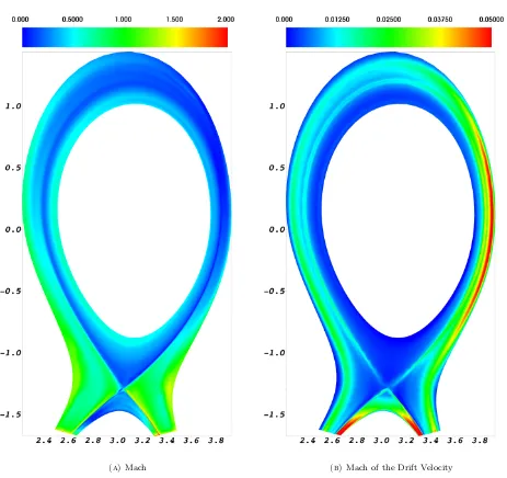
In the following plots the results of the simulation are shown. On the left and right side of Fig. 6 the u and n profiles of the computed solution are shown. The density results in logarithmic scale clearly show the presence of the separatrix : in the interior region the density is high while outside it quickly decreases near zero. The results for the parallel velocity clearly show how the flow is accelerated towards by the Bohm boundary conditions. Indeed in Fig. 7 the Mach number is shown. Fig. 7a shown the Mach number and again the strong acceleration due to the Bohm boundary conditions is obvious. Fig. 7b shows only the Mach number of the drift component of the velocity vector: this component is negligible almost everywhere except in the private flux region and in the weak field side where the magnetic poloidal field is stronger.
5.
Conclusions
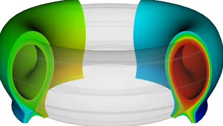
Figure 6. Computed results for the parallel velocity (left) and density (right) profiles, the
results for the density are in logarithmic scale.
that have the drawback to introduce curvature source terms in the continuous system of equation. Instead, this technique applies the discretization on the vector form of the equations where a strong conservation form does exist and then project the resulting discrete system on the basis of the curvilinear system defined on each control volume. Thus numerical methods have been validated on several simple test cases and applied on a 3D simulation of a reduced MHD model using the adiabatic assumption to express the electric potential. In the future, we plan to consider more complex MHD models and apply this method to the study of MHD instabilities and micro-turbulence in edge plasmas.
References
[1] A. Bonnement, T. Fajraoui, H. Guillard, M. Martin, A. Mouton, B. Nkonga, and A. Sangam. Finite volume method in curvilinear coordinates for hyperbolic conservation laws.ESAIM:PROCEEDINGS, 32:163–176, 2011.
[2] A. Harten, P.D. Lax, and B. van Leer. ”On upstreaming differencing and Godunov-type schemes for hyperbolic conservation laws”.SIAM Rev., 25:35–61, 1983.
[3] B. van Leer. ”Towards the ultimate conservative difference scheme V: a second-order sequel to Godunov’s method”.Journal of Computational Physics, 32(1):101–136, 1979.
[4] Jardins, S. ”Computational methods in plasma physics”.Chapman & Hall CRC, Computational sciences series, 2010. [5] Vinokur, M. ”Conservation equations of gasdynamics in curvilinear coordinate systems”.Journal of Computational Physics,
14:105–125, 1974.
(a)Mach (b)Mach of the Drift Velocity