Choosing the Best Bundle of Projects: A DEA Approach

Available online at http://ijdea.srbiau.ac.ir

Int. J. Data Envelopment Analysis (ISSN 2345-458X)

Vol.4, No.3, Year 2016 Article ID IJDEA-00422, 8 pages Research Article

Choosing the Best Bundle of Projects: A DEA

Approach

Mahnaz Mirbolouki

* (a)

Department of Mathematics, Yadegar-e-Imam Khomeini (RAH) Shahre Rey Branch,

Islamic Azad University, Tehran, Iran.

Received April 17, 2016, Accepted July 29, 2106

Abstract

One of the many important decisions organizations must make is project selection. Every project includes an initial plan to run, but not every plan can be implemented as a project. In situations where they lack resources or funds, all different plans must first be able to assess profitability in an accurate way, leading to the selection of a combination of proposals to carry out as projects. This paper provides a method to select the most effective set of proposals while considering the maximum use of available resources. Assessing efficiency is considered by a data envelopment analysis (DEA) model. Note that it is assumed that a vector of limited sources is at hand. This vector of resources can be contained human resource, budget, equipment, and facilities. Here, while reviewing some of the models in the selection project field, a common set of weight approach performance evaluation model for assessing the efficiency of the selected proposals is proposed. In this article it has tried to resolve the problems of former models.

Keywords: Data envelopment analysis; Efficiency; Project selection; Stochastic programming.

*. Email: [email protected]

1054 1. Introduction

Many researchers investigated the issue of selection proposals in various applications such as construction projects, portfolio selection, R&D proposals, location/ allocation problem, etc. Albino and Gravelli [1] proposed a neural network approach for subcontractor selection. They studied the neural network implementation and the related management and technical innovations by an application case related to an assembly operation in a construction site. Bhattacharyya et al. [2] presents a fuzzy multi-objective programming approach to facilitate decision making in the selection of R&D projects. Park et al. [9] considered preferences in National Institutes of Health (NIH) projects using natural experiment in research funding.

DEA was developed by Charnes et al. [4]. Nowadays, DEA is well-deployed in other industries with many papers published on its utilization for performance measurement and decision making. Several researchers using DEA models proposed several models to choose the best combination of projects with different objectives. Kumar et al. [8] studied six sigma projects and its analysis using DEA to identify projects, which result in maximum benefit. Maximum benefit here provides a Pareto optimal solution based on inputs and outputs directly related to the efficiency of the six sigma projects under study. Tavana et al. [10] have considered the problem of assessment and selection of high-technology projects at the National Aeronautic and Space Administration (NASA). They proposed a DEA model with uncertainty in input and output data, which is modeled with fuzzy sets. Their models are capable of maximizing the satisfaction level of the fuzzy objectives and efficiency scores, simultaneously. Moreover, these models are capable of generating a common set of multipliers for all projects in a single run. Chang and Lee [3] discussed the specific problem of selecting a portfolio of projects that achieves an organization’s objectives without exceeding limited capital resources, especially when each project possesses vague input and output data in the selection. In this paper, a DEA knapsack formulation and fuzzy set theory integrated

model was proposed. Cook and Green [5] investigated selection problem among a large set of proposals when there are some budget limitations. Their approach treats each subset of the projects that could feasibly be selected within the resource constraints as a single, composite project. These composite projects are then evaluated, by DEA.

Although the proposed model in this paper is similar to Cook and Green [5] paper in some details, it is different in the objective function. Also, in the special case where suggested proposals' income is imprecise stochastic DEA (SDEA) approach is proposed and deterministic equivalent is presented.

In this paper, we consider the problem of choosing appropriate combinations of proposals, which has the best efficiency measure. Assessing efficiency is considered by DEA and SDEA models.

Our approach is organized in five sections. In the following section preliminaries on efficiency evaluation by a DEA model is presented. Section 3 discusses the proposed model for deterministic data and section 4 is the extension of this problem for imprecise outputs of proposals. Section 5 is the conclusion.

2. Preliminaries

DEA is a non-parametric multi-factor productivity analysis model that evaluates the relative efficiencies of a homogenous set of decision-making units (DMUs) in the presence of multiple input and output factors.

Consider n homogeneous DMUs

; 1,...,

j

DMU j n, where each

j

D M U uses

input vector m

j

x R to produce output

vector s

j

y R . According to the DEA assumptions it is assumed that

0 , 0

j j

x y

 

  . Then the efficiency of

; {1, ..., } ;

o

D M U o  n by considering input

weights v _i,i 1, ...,m and output weights

,

1,...,

r

u r



s

is defined as follows:

1 1 2 2

1 1 2 2

...

...

o o s so

o

o o m m o

u y

u y

u y

E

v x

v x

v x









1055 To calculate input and output weights so that maximum relative efficiency of D M U_o

yields, Charnes et al. [4] proposed the following model:

1

1 1

1

m a x

. . 1,

1, ..., ,

, ,

1, ..., , 1, ..., .

r ro m i io i r rj m i i s r s r j r i i s t j n u u y v x v r i v m x s u y       _     









₍₁₎

where





0

is an infinitesimal value to avoid vanishing the weights. This linear fractional programming problem can be reduced to a non-ratio format in the usual manner of Charnes et al. [4] using transformation

1

1

m i i o i

v x







. Thus model (1) can be expressed as:

1

1 1

1

m a x

. .

0 , 1, ..., ,

, ,

1, ..., , 1, ..., 1 . , r ro m i io i m s r rj r

i i j s r r i i s t j n u v

r s i

u y

v x

u y v x

m              









(2)

The optimal objective of the above model, which is considered as the related efficiency of

o

D M U _{, ranges between zero and one.}

o

D M U _{is called an efficient DMU if it}

receives a score of one. Through using the method, there is no need to have the initial weight for the related inputs and outputs of every DMU. In the other words, the best input and output weights of each DMU are achieved through solving a linear programming problem in order to get a higher efficiency. The related efficiency of each DMU calculated by the method is higher than the actual real value. To overcome this difficulty, the following model was proposed, which determines a set of optimal weights for all DMUs:

max 1, 2, ,

1 1 1 1

1 2

1u yr r u yr r 1u yr rn

m m m

v x v x v x

i i i i i i i i in

s s s

r r r

 _  _   _  _  _ 













. . 1 1 1, ..., ,

1

ε, 1, ...,

ε, 1, ...,

s t

u y_{r rn} m _{v x} i i in u s r r s r v j n i m i           (3)

The aim of this model is to determine a common set of weights to get the highest efficiency of all DMUs simultaneously. Model (3) is a multiple objective problem. There are some approaches to solve this model. Hosseinzadeh-Lotfi et al. [7] linearized model (3) using a goal programming approach, which minimizes the sum of deviations from the efficiency level. This model is as follows:

min ₁

1 1

. .

1, ..., ,

0, 1, ..., , ε, 1, ..., ,

ε, 1,.. , ., . =0 n j j

s _{u y} m _{v x}

r r rj i i ij j

s t

j n

j n

j

u_r r s

v_i i m

      _  _         (4)

Suppose



* * *



, ,

u v  is an optimal solution of model (4), then the efficiency score of

j

D M U can be calculated using the following expression:

* *

1 *

1 , 1,...,

* *

1 1

s _{u y}

r r rj j

j n

j _{m m}

v x v x i i ij i i ij



     

_ _

(5)

3. Choosing the best subset of proposals In this section we assume every proposal, which requests m types of resources to produce s types of outputs, as a DMU. Also, a manager encounter with the problem of choosing the most efficient subset of proposals with the following limitation on the available resources:

1056 (b)The remaining resources after allocation to the final selected set;

S

*, must be too little to allow other proposals into

S

*.

For this purpose, assume binary variable

k

_j which take the value 1 if proposal j is selected to implement and zero otherwise. Consider the following constraints which are proposed by Cook and Green [5]:

, 1

n _{k x s b i}

j j ij i i

 _    (6)

(1 )

1 _,

k x M k M h j ij j ij s_{i M} i j

   

  

(7)

1 1

m _{h m j}

i ij

 _    (8)

Where M is considered as a big number. The constraints (6)-(8) satisfy both assumptions (a) and (b). If k _j 1 then constrains (7) are obviously satisfied. In the situation that

0

j

k  and x_ij  s_i , constraints (6) and (7) result h_ij 1, on the other hand x_ij  s_i

results

h

_ij



0.

Constraints (8) lead to condition (b), since if 0

j

k  , this constraint assure that at least

one of h_1j,h_2j,...,h_{m j} gets zero value, which means that a not selected proposal could not be implemented by the remaining resources.

Now, consider the modified version of model (3), which contains the binary variables

k

_j

'

s

and resource constraints (6)-(8):

1 2

max ₁ , ₂ , ,

1 1 1 1 1 1 2 1

u y_{r r} u y_{r r} u y_{r rn}

k k _kn

m _{v x} m _{v x} m

s s s

v x i i i i i

r r r

i i i in

            













1

, 1, ..., , (9 .1) 1

1

(1 )

1, ..., , 1, ...

. . 1, 1, ...

, ,

, ,

2 1

. ( 9 )

s r

n _{k x s b i m} j j ij i i

k _j x_ij M k _j M h_ij s_{i M} i m j n

u_ry_rj

s t k _j j n

m _{v x} i i ij

   _              

















1, 1, ..., 1

1, ..., , 1, ..., , ( 9 .4 )

0 , 1, ..., , ( 9 .5 )

, 1, ...,

, { 0 ,

, 1, .. 1}

ε ., .

,

,

m _{h m j n}

i ij

i m j n

s i

k _j h_ij

u r

m i

v_i r s i m

 _            (9)

Model (9) is a nonlinear MIP model. This model can be converted to the following linear MIP model:

1

. . k 1,...

max

0

1 1 , ,

n

j j

s m

s t _{r j}u y_{r rj i} k v x_{j i ij j} j n





 

 _ _   

0, 1,..., , , 1,..., , , 1,..., , (9.1) (9.5).

j n

j

u_r r s

v_i i m

          (10)

The above model, which calculates the most efficient proposals, can be applied on many applications. Despite the applicability of the model, it cannot be applied when inputs and outputs of proposals are imprecise. In the next section, the extension of model (10) into a chance constrained programming model is presented where deterministic inputs against imprecise outputs are assumed. This assumption may be accrued in many real word applications such as construction projects, portfolio selections, urban development and etc. Each proposal has an opportunity to participate in the ‘production possibility set’ as well as to combine with other projects to be evaluated against possible technology and to be selected.

4. Selecting strategy for proposals with imprecise income

1057 Let's assume related outputs of

j

D M U have normal random distributions as,

2

( , )

rj rj rj

y  N y 

Then, the probabilistic form of the first constraint of model (10) can be stated as the following chance constrained approach:



s 1 m1 0



1

P _ru y_{rj rj} _iv x_{ij ij} _j    (11)

Where



is the level of error between zero and one. According to statistical rules, the left hand-side of inequality (11) gets the zero value. To make this inequality meaningful, by removing variable



_j it can be changed to the following:



s ₁ m₁ 0



1

P _ru_{rj rj}y _iv x_{ij ij}   (12)

Now defining random variable

1

s

j _r rj rj

h 



_u y , would be result the following deterministic constraints:

 

1

1 1 0

s m

u y v x s

r rj rj i ij ij j  j



 

 _  _   

y 2

1 1u u Covrj tj (yrj, )

s s

r t

j tj

  _  _   (13)

Where  is the cumulative distribution function of the standard normal distribution and 1_{ }

 , is its inverse in level of α.

Also, 1_{ }

j

 



 indicates the deviation

from stochastic frontier with respect to α level of error and

s

_j is an alternative of



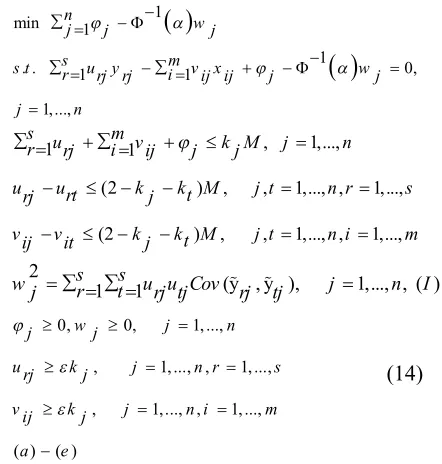
_j.

Finally, the deterministic equivalent of the related chance constraint model (10) can be written as,

 

 

1 1 0 min ₁

. . _{1 1}

1 , ,..., n j j s m

s t _r u_r y _i v x w j

j rj ij ij j

j w n j      _               1,..., 1 1

, 1,..., , 1,...,

, 1,..., , 1,... ,

(2 ) ,

(2 ) , ,

u_rj u_rt k_j k_t M v k k_t M ij

s _u m _{v k M j n} r i

it j

rj ij j j

j t n r s

v j t n i m

  _  _                 2

(y , y ), 1,..., , ( )

1 1

w_j s_r _ts_u u Cov_{rj tj} _rj _tj j  n I

1, ...,

, 1, ..., , 1, ...,

, 1,..., , 1, ...,

( ) ( )

0, 0, j n j

u_rj k_j j n r s

v_ij k j n i m

w e j j a              (14)

In the model (14) constraints (a)-(e) are the same constraints in model (10) and constraints (I) make this model nonlinear.

Example 1. (a numerical example)

Consider eight DMUs with two inputs and one probabilistic output. Table 1 contains the related data of these DMUs. Now we are going to select the best combination of these DMUs in the limited resources condition. In this example it is assumed that the each DMU's output is normally distributed. The example is solved at the levels 5% and 60% of error by the model (14) and the results are shown in table 2. The results in table 2 show that when the error level is decreased the proper use of resources would be gain. Notation '-' in table2 is for unselected DMUs.

Table 1. inputs and output

1058

Table 2. Computationally results of model (14)

60% error 5% error

input2 input1

input2 input1

9 7

- -

DMU1

8 5

- -

DMU2

- -

4 10

DMU3

- -

- -

DMU4

- -

- -

DMU5

- -

3 14

DMU6

6 7

- -

DMU7

- -

13 8

DMU8

2 19

2 3

Remained Resource

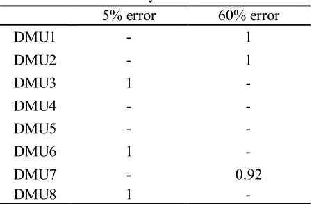
The efficiency of the selected DMUs in each level of error is demonstrated in table 3. The

results of this table indicate more efficient selection in lower error.

Table 3. efficiency of each selection

60% error 5% error

1 -

DMU1

1 -

DMU2

- 1

DMU3

- -

DMU4

- -

DMU5

- 1

DMU6

0.92 -

DMU7

- 1

DMU8

5. Conclusion

In this paper, a MIP model is offered in order to optimize the selection of the most efficient and feasible subset of proposals. In this way, the amount of deviation from efficiency level is minimized. The issue of the choice of this efficient bunch is one of the issues raised in many of the organizations that their practical projects encounter with the lots of suggestions, while the lack of funds prevents them from implementing all those projects. In this paper the selection project is considered in two conditions. First considering all inputs and outputs deterministic and second considering imprecise income for projects. The second

assumption is more compatible with many real world applications such as portfolio selection where the result of investment never is clear. The results of the numerical example in section 4 confirm the maximum use of existing resources and the efficient selected bundle.

Acknowledgment

1059 References

[1] Albino, V., and Gravelli, A., A Neural Network Application to Subcontractor Rating in Construction Firms. Int. J. Proj. Manag., 1998, 16 (1), 9-14.

[2] Bhattacharyya, R., Kumar, P., and Kar, S., Fuzzy R&D portfolio selection of interdependent projects. Comput. Math. Appl., 2011, 62(10), 3857-3870.

[3] Chang, P. T., and Lee, J. H., A fuzzy DEA and knapsack formulation integrated model for project selection. Comput. Oper. Res., 2012, 39, 112-125.

[4] Charnes, A., Cooper, W. W., and Rhodes, E., Measuring the efficiency of decision making units. Eur. J. Oper. Res., 1978, 2, 429-444.

[5] Cook, W. D., and Green, R. H., Project prioritization: a resource-constrained data envelopment analysis approach. Socio Econ. Plan. Sci., 2000, 34, 85-99.

[6] El-Mashaleh, M. S., A Construction Subcontractor Selection Model. Jordan J. Civil Eng., 2009, 3(4), 375-383.

[7] Hosseinzadeh-Lotfi, F., Hatami-Marbini, A., Agrell, P.J., Aghayi, N., Gholami, K. Allocating fixed resources and setting targets using a common-weights DEA approach,

Comput. Ind. Eng., 2013, 64, 631-640.

[8] Kumar, U. D., Saranga, H., Ramírez-Márquez, J. E., and Nowicki, D., Six sigma project selection using data envelopment analysis, TQM Mag., 2007, 19(5), 419-441.

[9] Park, H., Lee, J., and Kim, B. C., Project selection in NIH: A natural experiment from ARRA. Res. Policy, 2015, 44, 1145-1159. [10]Tavana, M., Khalili-Damghani, K., and Sadi-Nezhad, S., A fuzzy group data