AUT J. Elec. Eng., 49(1)(2017)95-106 DOI: 10.22060/eej.2017.12053.5029
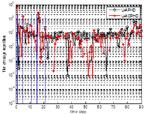
Unscented Auxiliary Particle Filter Implementation of the Cardinalized Probability
Hypothesis Density Filter
M. R. Danaee1 and F. Behnia2
1 Electrical Engineering Department, Imam Hossein Comprehensive University (IHCU), Tehran, Iran 2 Electrical Engineering Department, Sharif University of Technology, Tehran, Iran
ABSTRACT: The probability hypothesis density (PHD) filter suffers from lack of precise estimation of the expected number of targets. The Cardinalized PHD (CPHD) recursion, as a generalization of the PHD recursion, remedies this flaw and simultaneously propagates the intensity function and the posterior cardinality distribution. While there are a few new approaches to enhance the Sequential Monte Carlo (SMC) implementation of the PHD filter, current SMC implementation for the CPHD filter is limited to choose only state transition density as a proposal distribution. In this paper, we propose an auxiliary particle implementation of the CPHD filter by estimating the linear functionals in the elementary symmetric functions based on the unscented transform (UT). Numerical simulation results indicate that our proposed algorithm outperforms both the SMC-CPHD filter and the auxiliary particle implementation of the PHD filter in difficult situations with high clutter. We also compare our proposed algorithm with its counterparts in terms of other metrics, such as run times and sensitivity to new target appearance.
Review History:
Received: 17 October 2016 Revised: 4 February 2017 Accepted: 27 February 2017 Available Online: 2 March 2017
Keywords:
Multi-target tracking
Cardinalized probability hypothesis
density filter
unscented auxiliary particle filter
linear functional potential functions
1- Introduction
In the context of the multi-target tracking (MTT), we have to estimate the set of unknown target states and its time-varying cardinality. Mahler provides an excellent context to cope with these difficulties. This is done by introducing the concept of finite set statistics (FISST) [1-3]. The major drawback of the FISST Bayes filter is facing manifold integrals of the multi target states in high dimensional space, which makes practical implementations of tracking system impossible. A first moment approximation to the full multi-target Bayes recursion, namely the probability hypothesis density (PHD), is introduced by Mahler [4] to propagate the posterior intensity function rather than the multi-target posterior density in time and reduce computational expense [4].
In order to emerge higher moment information into the PHD recursion, Mahler suggested a generalization of the PHD filter named the cardinalized PHD (CPHD) filter which simultaneously propagates the cardinality distribution together with the intensity function [5, 6]. There are many application areas for this powerful filtering strategy such as image tracking [7], sonar [8] , extended target tracking [9], and data fusion [10, 11]. Recently, the CPHD filter is applied in the distributed multi-sensor tracking where sensors share their incomplete knowledge of moving targets and help each other to improve the estimation of targets’ state vector [12,13]. The sequential Monte Carlo (SMC) implementation of the PHD and CPHD filters are first introduced in [2, 14, 15] using state transition density as a proposal distribution. Consequently, there are a few attempts made to enhance the SMC implementation of the PHD filter [16-18]. However, despite the supposed superiority of the CPHD over the PHD
filter, to the best knowledge of the author, there is no apparently parallel approach for the auxiliary particle implementation of the CPHD filter. This is because the CPHD filter has more complex recursion compared to the PHD filter. Our goal is to make this filter efficiently implemented by exploiting the state-of-art auxiliary variable particle filtering (AVPF) algorithm and this paper is an extension to our previous work [19]. However, the main difference between this paper and previous work [19] is our focus on construction of proposal distributions. In this paper, in order to design proposal distributions, we pay attention to the relation of newly born targets with both detected and undetected target spaces. The spaces for newly born and persistent targets are explored more rigorously by using potential functions to generate more promising particles.
this filter outperforms its counterparts both in cardinality estimation and localization accuracy, even in harsh situations such as in scenarios with high clutter.
The structure of this paper is as follows. The CPHD recursion is introduced in Section II. The implementation of the CPHD filter based on the idea of the auxiliary particle filter is described in Section III. The application of UT for construction of the proposal distributions is discussed in Section IV. In Section V, through a simulation scenario of MTT with various clutter levels, the performance of our proposed algorithm is evaluated in terms of different metrics and compared with counterpart algorithms. Closing remarks are given in Section VI.
2- Cardinalized Phd Filter
According to finite set statistics (FISST) framework, which is the appropriate formulation of the point process theory [20] in MTT application, the multi-target state is represented as a finite set X={x1,..., xn} with target state-vectors x1,..., xn and random target number n. So the state X is a random finite set . Mahler [4], analogous to constant-gain Kalman filter, developed a first-order statistical moment of the full multi-target probability density which is named the probability hypothesis density (PHD)
where dw(x) denotes the Dirac delta function concentrated at w. The PHD filter serves as a powerful technique for decluttering. However, [21] argues that estimating the number of targets, the merit obtained by using the PHD filter, is subject to a large variance due to propagation of only the first-order statistical moment of the full target posterior distribution.
To that end, [5] proposed cardinalized PHD (CPHD), which propagates not only PHD but also the whole probability distribution on the number of targets. The prediction and correction steps of the CPHD filter are given by the following section.
A. CPHD Prediction
The intensity function Dkk(xk) is forwarded in time by retaining survived targets (persistent targets) as well as adding newly born targets
where we extend the state space E of the survived target with dimension d, E⊂Rd by an isolated ‘source’ point S, representing a state space of newly born target, so that we may denote by E` the extended space E∪{S}. Individual targets evolve independently according to the extended single-state Markov transition density
where b(x) is the birth intensity function, which in this paper follows the Gaussian distribution defined as
where gb is the predicted number of newly born targets at each time-step and mb is the state vector of a newly born target most likely to appear in the observation area, and Qb is the uncertainty covariance matrix.1 Furthermore, b[h] is the corresponding linear functional of the function h(x) and defined as
1 We can also apply a Gaussian mixture for b(x) , when the initial position of a newly born target is a multimodal distribution.
Consider a target with the x and y positions [xk,yk], corresponding velocities [vx,k,vy,k] and the turn rate wk. We assume that the target trajectories are modeled by nonlinear nearly-constant turn model [22] to represent f(xk+1|xk). That model describes the evolution of the target state xk=[xk,vx,k,yk,vy,k,wk]` as
where the process noise ek has a multivariate normal
distribution defined as with
and T is the sampling time. As a result, we may write
The extended probability of survival for a target with state xk at time-step k is given by
where ps(xk) is the survival probability of the persistent target with state xk. We also denote by the extended intensity function defined as
The prediction cardinality distribution is given by
where pB(n) is the cardinality distribution of newly born targets, G(x)=Gk|k(x) is the probability generating function (PGF) of the cardinality distribution of fk|k(X|Z(k)),
where , and Note that G(i)(x) is the derivative of G(x).
B. CPHD Correction
At time-step k+1 we receive measurements which comprise a finite set Zk+1={z1,...,zm}. Those measurements belonging to the true targets are generated based on the range and bearing measurement model
where vr and vq are zero mean Gaussian measurement noises of variance s2
r and s2q respectively. Furthermore, we adopt the notation Z(k+1)=Z
1,...,Zk+1. The measurements which do not belong to true targets are false alarm events which we assume that they are Poisson processes with spatial distribution c(z) and average number of clutter points l.
Each target is detected with the probability of detection pD(x). The correction step of the CPHD filter is given by
X
(1)
(4)
(5)
(6)
(7)
(8) (2)
(3)
( )
| x
a k k k
D
( )
(
)
( )(
[ ]
)
[ ]
1|
0
1
. . 1 .
!
n i
i
k k B S S
i
p n p n i G s p s p
i
+
=
=
å
--[ ]
( ) ( )
x x xs h =
ò
h s d ( )(
)
| | x| k x
k k k k
N =
ò
D Z d[
]
{
}
(
)
2 2
2 2
arctan
,
=
r r
r r
y
v
z
x
y
v
x
v
R E
v
v
v
diag
q
q q
q
s s
¢
é
æ ö
ç
÷
ù
é ù
ê
ú
=
ê
+
ç ÷
ç
è ø
÷
ú
+
ê ú
ê ú
ë û
ë
û
é ù
=
ê ú
ê ú
ë û
( )
( )
X( ) ( )
D xX EéëdX x ù =û
ò
d x f X X Xd(
)
(
)
( )
( )
1| 1 a 1| a a|
k k k E k k S k k k k k D + x + f x + x p x D x dx
¢
=
ò
× ×(
)
(
(
1) [ ]
)
1
1
/ 1
|
|
k k ka k k
k k
f x
x
x
E
f x
x
b x
+b
x
S
+
+
ìï
Î
ï
= í
=
ïïî
( ) b ( ; ,b b),
b x =g × x m Q
( ) ( )
[ ] .
b h = òh x b x dx
( )
( ) ( ( ))
( ) ( )
( )
( ) ( )
( ) ( )
2
2 1
1 sin / 0 1 cos / 0
0 cos 0 sin 0
0 1 cos / 1 sin / 0
0 sin 0 cos 0
0 0 0 0 1
/ 2 0 0
0 0
0 / 2 0
0 0
0 0 1
k k k k
k k
k k k k
k k
k
k k k k
k
w T w w T w
w T w T
w T w w T w
w T w T
T T
T T
x F w x G
x
+
× - - ×
× - ×
- × ×
× ×
+ ×
= × + × =
é ù
ê ú
ê ú
=ê ú×
ê ú
ê ú
ë û
é ù
ê ú
ê ú
ê ú
ê ú
ê ú
ë û
e
e
(×;0 ,3 1´ Q)
Q diag=
(
s s se2, ,e2 w2)
(
k 1| k)
(
k 1;( )
k k,)
.f x + x = x + F w ×x G Q G× × ¢
( )
{
S( )
1
k k.
a k
S
k
p x
x
E
p x
=
x
Î
=
S
( )
[ ] ( )
|( )
|
1
.
a k S k k k k
k k
D
x
=
b
d
x
+
D
x
( )
1 |( )
where we denote
where Lzp(x)=f(zp|x) is the measurement likelihood function. We denote qD(x)=1−pD(x). In addition, we define the function as
where pk(n) is the cardinality distribution of false alarms, p(n)=pk+1|k(n) is the predicted cardinality distribution at time-step k+1, Pkn is the k-permutations of n, and si(Z) is given by
where the elementary symmetric function sm,i(y1,...,ym) of degree i in y1,...,ym is given by
where the degree zero is given by convention as
and we denote by
We assume that pD(x) is independent of state-vector x for all x and we may, therefore, write s[qD]=qD.
Consequently, the cardinality distribution is updated in terms of the predicted cardinality distribution as
3- Auxiliary Particle Filter Implementation
To convey the idea behind our proposed approach, we first consider a discrete approximation of the following integral
by using samples generated from a proposal distribution, where j is a test function. Instead of forwarding all existing particles with an inefficient proposal distribution such as
fa(x
k+1|xk), we may construct an efficient proposal distribution. We achieve this goal by using auxiliary particle filter principle and sampling on a higher dimensional space in the hope that it will increase estimation accuracy. The principle of the Auxiliary Particle Filter (APF) [23], which is using auxiliary random variables may be applied in the target tracking contexts in which the number of targets are not already known and can be changed during the time.
The application of the auxiliary random variable can be extended for detection and tracking a target within raw measurements [24] or multiple target tracking using the PHD filter with time varying number of targets [17] .
We explore a situation in which targets are detected by probability density which are defined on spaces E×E`×|Zk+1|. In this situation, auxiliary variables include existing particles and indices of current measurements p∈{1,...,|Zk+1|}. Consequently, sampling on a higher dimensional space is done by first picking up a measurement which can be regarded as an observation more probably generated from a true target. Secondly, we select an existing particle on the basis of how well it describes the picked up measurement. We also explore a situation of undetected targets by proposal distribution defined on spaces E×E` by using existing particles as auxiliary variables.
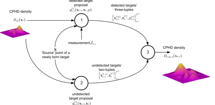
The fundamental flow of the Auxiliary CPHD (ACPHD) algorithm is shown in Fig. 1. Based on the source point of a newly born target, existing particles which are approximating Dk|k(xk), and current measurement set Zk+1, N(1) three-tuples are sampled while the super script d in denotes samples belong to detected targets. For undetected targets, draws N(2) two-tuples where while the super script m in denotes samples belong to undetected targets. We take the union of these Np=N(1)+N(2) tuples with their corresponding importance weights as the discrete approximation of Dk+1|k+1(xk+1).
We substitute Dk+1|k+1(xk+1) appeared in (17) with its comprising terms defined in (2) and (9), and then we use the proposal distributions in order to change the integrand in (17) to
According to the Bayes’ rule, we can decompose the joint proposal distributions as
(9) (10) (11) (12) (13) (14) (15) (16) (18) (17)
( )
u Z ¡ ( )(
)
( )(
)
( ) ( ) ( ) 0 1| ! . .. P . . ,
Z
u k j
j u j
k k n j u n
D j u n j u
Z j
Z p Z j Z
N
q p n
s + = + ¥ - + + = +
-¡ =
å
-å
( ) [ ] ( ) [ ] ( ) 1 1| 1| ,1 , , ,
z z
z z
m
k k D k k D i m i
m
D p L D p L
Z
c c
s s æççç + + ö÷÷÷ ÷÷ çè ø ( ) , 1 , , , ,
m i m j
j S S U S i
y y y
s
Î
Í =
=
å Õ
(
)
,0 1
, ,
1,
m
y
y
ms
=
[ ]
1|
k k D + h
( ) ( ( )) ( ) ( ) ( ) ( ) 1 1| 1| 1 0 1
1 1 1
0 1| !. . . .P . k k k k k k Z
k k k j k
j n j D n j j k k p n p n Z
Z j p Z i Z
q N s + + + + + + + + = -+ = ¡
æ - - ö÷
ç ÷ ç ÷ ç ÷ ç ÷ ç ÷ ç ÷÷ ç ÷ ç ÷ ç ÷ çè ø
å
( )
1( )
( )
1| 1 k
.
1|k k Z k k
D
+ +x
@
L
+x D
+x
( )
( )
( )
( )
( )
( )
( )
(
( )
{ }
)
1 0 1 0 1 .. zp . ,
Z D Z p D p p Z
L x q x
Z
Z z L x
p x
c z Z
= ¡ ¡
æ ¡ - ö÷
ç ÷
ç
+ çç ÷÷
¡ ÷ çè ø
å
[ ]
( ) ( )
1| 1| . k k k k D hD x h x dx
+
+ =
ò
(
k 1)
k 1|k 1(
k 1)
k 1E
x
D
x
dx
j
=
ò
j
+ + + + +( )1
(
)
11 k , ,k
k
q + x + x p
1
{ }n Np n k
x =
( )2 1
1( k , k)
k
q + x + x
1
{ }n Np n k
x =
1
{ }n Np n k
x =
( ) ( ) ( ) ( )1
,
1
1 1
{ d n , in , n }N n
k k k
x + x p + =
( ) , 1 d n k x +
( )2
(
)
11 k , k
k
q + x + x ( ) ( ) ( )2
,
1 1
{
m n,
in}
Nn k k
x
+x
= xkm n+,( )1( )1
(
)
( )2(
)
1 1
1 k , ,k 1 k , k
k k
q + x + x p and q + x + x
( ) ( ( )) ( ) { }
(
)
( ) ( ) ( ) ( ) ( ) ( ) 1 1 1 1 1 1 1 0 1 1 | 1 1 1 . . | , , z k p ZD k k
k
p p E E
p k
k
a a
a k k S k k k k k k k x x x z z
x x x x
x x
p L
c Z
Z
f p D
q p
j + j + + +
= ¢ + + + + + = ¡ -´ ¡ × × ´
å ò ò
( ) ( ) ( )
(
( ))
(( )) ( ) ( ) ( ) ( )( ) ( )( ) 1 | 2 1 1 2 1 1 1 1 1 1 1 1 11 1 0
1 , | , , . ,
. 1 .
a a
a k k k k
S k k k k k
k k k k k
k k k k k k D k k k E E
x x p x x
x x
f x x p x D x
q x x
q x x dx dx
q d d
and
We can also trivially prove that the minimum variance of importance weights is direct consequence of the following choices of decompositions
where and are bounded potential functions for detected and undetected targets respectively, and defined as follows
We apply the potential function to enforce current measurement’s fitness on the selection of xk, while can determine how likely the existing particle xk is to be undetected at the time-step k+1 Estimations of these potential functions by both UT method (in prediction mode) and drawn samples (in update mode) are the key elements of our algorithms. This is due to the fact that, as we will show later on in the paper,
other parameters can be readily computed based on these potential functions.
Now suppose that, we have a discrete approximation of the CPHD filter at time-step k with a limited number of particles and related weights
and therefore
These approximations become exact when the number of particles grows to infinity. Based on the discrete approximation in (27), the equations from (21) to (23) are adjusted as
4- Application Of UT To Auxiliary CPHD Filter
In order to build the proposal distributions for sampling auxiliary variables, we have to determines integrals (24) and (25). However, it is generally impossible because new samples xk+1 are not yet available. Here, we can use the unscented transform to approximate the values of the potential functions based on the existing particles rather than resorting to unknown samples xk+1.
measurement, detected target proposal undetected target proposal 1 2 3 CPHD density ( ) ( ) ( )
{
}
( )1,
1 1
1
, in, N
d n n
k k k
n p + + = x x detected targets’ three-tuples ) ( )
{
}
( )2, 1
1
, in N
m n k k n + = x x undetected targets’ two-tuples 1 k Z+
‘Source’ point of a newly born target
( )1 ( ) 1 1 k , ,k k
q+ x x+ p
( )2( 1 ) 1 k ,k k
q+ x x+
( )
| k k k
D x
CPHD density ( 1)
1| 1 k k k
D+ + x+
S
Fig. 1. Auxiliary CPHD algorithm implementation. Two proposal distributions (for detected targets) and (for undetected targets) generate samples to approximate .
( )1 ( )
1 1 xk , ,xk k
q + + p
( )2 ( )
1 1 xk ,xk k
q + + Dk+1|k+1(xk+1)
(19) (20) (21) (26) (27) (28) (29) (30) (22) (23) (24) (25)
( )1 ( ) 1, xk k+ p
k( )+21
( )
xk( ) ( )
1
{xn , n N} p
n k wk =
( )
(
)
( )(
)
( )(
)
( )( )
1 1 1 1 1 1 1 1 1 1 , , , | , |k k k k
k k
k
k k
q x x p q x x p
q x p q p
+ +
+ +
+ +
=
´ ×
( )2
(
)
( )2(
)
( )2( )
1 1
1 k , k 1 k | k 1 k .
k k k
q + x + x =q + x + x ×q + x
( ) ( )
(
{ })
( ) ( ) ( ) ( ) 1 1 1 1 1 11, | , 1, , ,
k p
k
p a
k k k k
k p k k E
Z z
q p
c z
x D x dx p Z
+ + + + ¢ ¡ -µ
´
ò
× = ( )
(
)
( )( )
( )
( )( )
( )
1 1, | 1 1 1 1, || k p k k ka k ,
k
k a
k k k
k p k k
E
x D x
q x p
x D x dx
+ + + ¢ × = ×
ò
( )( )
( )( )
( )
( )( )
( )
2 1 | 2 1 2 1 |,
a k kk k k
k k
a
k k k
k k k
E
x
D
x
q
x
x
D
x dx
+ + + ¢
×
=
×
ò
( )( )
(
)
(
)
(
)
( )
1 1 1 1,1| 1,
p
k D k z k
k p
E a
a k k k k
S
x p x L x
f x x p x dx
+ + + + + = × × ´ ×
ò
( )( )
(
(
)
)
(
)
( )
2 1 1 1 11
|
.
k D k
k
E a
a k k k k
S
x
p x
f x
x
p x dx
+ + + +
=
-´
×
ò
( )1 ( ) 1, k k+ p x
( )2
( )
1 k k+ x
( )
( )( )
( )
| p1 i ,
k N i
k k k i k x k D x =
å
=w ×d x( )
|( )
[ ] ( )
| 1 .
a k k k k k
k k
D x =D x +b dS x
( )
( )
(
{ }
)
( )
( )( )
( ) ( ) ( )( ) [ ]
(
)
1 1 1 1 1 1 1, 1,1 1 ,
p
k p
k
p
N i i
k p k k k p i
Z z
q p
c z
x w S b
+ + + + = ¡ -µ
´
å
× + ×( ) ( ) ( )
( )
( ) ( ) ( )( ) ( )( )
( ) ( ) ( ) ( ) [ ] ( ) ( ) [ ] ( ) ( )( )
( ) ( ) ( ) ( ) [ ] 1 1, 1 11 1 1
1, 1, 1 1 1, 1 1 1, 1, 1 | 1 1 , 1 S p i k p p
N i i
k k p k k x i
k
k N i i
k p k k k p i
k k p
N i i
k p k k k p i
x w x
q x p
x w S b
S b x
x w S b
d d + = + + + = + + + = × × = × + × + × × + × + ×
å
å
å
( ) ( ) ( )( )
( ) ( ) ( )( ) ( )( )
( ) ( ) ( )( ) [ ] ( )( ) [ ] ( ) ( )( )
( ) ( ) ( )( ) [ ] 2 1 2 11 2 2
1 1 1 2 1 2 2 1 1 1 1 1 . 1 S p i k p p
N i i
k k k k x i
k
k N i i
k k k k
i
k k
N i i
k k k k
i
x w x
q x
x w S b
S b x
x w S b
d d + = + + + = + + + = × × = × + × + × × + × + ×
å
å
å
{ }
n Np1 k nOne of the benefits of applying UT is that its byproducts can be used to design Gaussian proposal distributions
For each sample xk(i) we keep track of a posterior covariance matrix Pk(i), so that we form augmented state vector, , and covariance, , with zero mean noises ek and xk as
where Q and R are defined in Section II. For the newly born target sample , we should define an augmented state vector and a covariance with different dimensions as follow
where mb and Qb are mean and covariance of the birth intensity function and is a covariance matrix that expresses the uncertainty about the mean of the distribution of newly born targets, so that sb could be a very small positive value.
We build a matrix of 2L+1 UT sigma points (vectors) to capture statistics of the stochastic process of target motion defined via the nonlinear transformation in (4) as
where L is the dimension of the augmented state and
is a scaling parameter with a secondary scaling parameters k and a . Relating UT weights are defined according to
where b is a constant.
Going for the time update, we form the jth predicted sigma point state, as
where we denote by c(:,j) the jth column of c and by c(a:b,j) the jth column of c where the number of its rows goes from a to b. Note that c(5,j) particularly denotes the turn rate of c(:,j). The predicted sigma point states of (35) play a key role in approximating the potential functions. We denote by
the predicted estimate of the potential function which is computed as
The predicted estimate of potential function for the case of undetected targets, , can be computed analytically if the detection probability is independent of a target state (and in this paper we assume the same property for all states). As a result, (25) is simplified to the following form
and thus there is no need to apply UT anymore.
Similar to the previous notation for , we denote by the predicted estimate of the linear functional
, where we replace with
Now it is possible to construct the proposal distributions for sampling auxiliary variables of detected targets
where is defined in the same way as U1(Z
k+1−{zp}), expect that Dk+1|k[pDLzp] is replaced by the predicted estimates
for p=1,...,|Zk+1. The function U1(Zk+1−{zp}) is also defined in terms of the bounded potential functions. To see that, let’s look at (11) which shows that U1(Z
k+1−{zp}) is a function of sj(Zk+1−{zp}) for j=1,...,|Zk+1 .p=1,...,|Zk+1 These elementary symmetric functions, in turn, need the quantity of Dk+1|k[pDLzp], p=1,...,|Zk+1 which are the corresponding linear functional of the predicted intensity function, Dk+1|k(xk+1), and defined as
Now let the respective sample-based approximation of Dk+1|k(xk+1) be
(31) (36) (37) (39) (40) (38) (32) (33) (34) (35) ( ) ,
xa i k
( )
,
Pa i k
( 1) xNp S
k + =
2 I5 5
b
s × ´
( ) , a i k c
(
)
2 L L
g a= + -k
( ) ( ) ( ) ( ) ( )
( ) ( ) ( )
2
0 / , 0 / 1
0.5 / , 1, ,2
m c
m c
j j
W L W L
W W L j L
l l l l a b
l
= + = + + - +
= = + =
( ) ( ) 1| :, 5 1
x i k+k j ´
c
( )1 ( ) 1,
ˆˆ ( )xi k+ p k
( )1 ( )
1, ( )xi
k+ p k
( )2 ( )
1
ˆˆ ( )xi k+ k
( )1 ( )
1,
ˆˆ ( )xi k+ p k
1|
ˆˆ [k k D zp]
D + p L
1| [ zp] k k D
D + p L k( )+11,p( )x( )ki ˆˆ ( )k( )+11,p x( )ki
1 1
ˆˆ (Zk+ { })zp
¡
-[ ]
1|
ˆˆk k D zp
D + p L
( )1
(
)
1 1
1 k | k, , 1, , k k
q + x + x p p= Z +
( ) ( ) ( )
( )
5 3 5 2 ,
, 1 3 1 2 3 5 3 2
2 5 2 3
0 0
0 0 , 0 0
0 0
, 1, , ,
i k
i i a i
a
k k k
p
P
x x P Q
R i N ´ ´ ´ ´ ´ ´ ´ ´ é ù ê ú ¢ é ù
=êë úû = êê úú
ë û
=
( )
[
]
( )
1
, 1 5 1 2
2 5 5 5 5 5 2
1
, 5 5 5 2
2 5 2 5
0 0 ,
0 0
0 0 ,
0 0 p p N a b k b N
ak b
x m I P Q R s + ´ ´ ´ ´ ´ + ´ ´ ´ ´ ¢ =
é × ù
ê ú
= ê ú
ê ú ë û ( ) ( ) ( ) ( ) ( ) ( ) , , , , 2 1
a i a i a i a i
k k k k
L L
x x L P
c l
´ +
é ù
=êë ± + úû
( )
( )
( )(
)
(
)
( )(
)
( )(
)
( )(
)
( )(
)
,1| 5 1
, ,
,
, ,
:,
5,
.
1:5,
6 :8, ,
0, ,2 ,
1, ,
1:5,
6 :10, ,
0, ,2 ,
1
x i k k
a i a i
k k
a i k
p
a i a i
k k
p
j
F
j
j
G
j
j
L i
N
j
j
j
L i
N
c
c
c
c
c
c
+ ´=
ìïï
ïï
ïï
+ ×
ïï
í
= ¼
= ¼
ïï
ï
+
ïï
ïï
= ¼
=
+
ïî
( )
( )
( )(
( )( )
)
(
( )( )
)
( )( )
(
)
( )2
1 , ,
1, 0 1| 1|
, 1|
ˆˆ :, :,
:, , 1, , 1
p
L
i a x i x i
D S
k p k j k k k k
x i m
z k k j p
x p j p j
L j W i N
c c
c
+ = + +
+
= ×
´ × = ¼ +
å
( )2
( )
{
(
)
1 k
1
1
D S kk k
D
p
p
x
S
x
p
x
S
+
=
-
-
×
¹
=
( ) ( ){
}
(
)
(
)
{ }(
)
( ) ( )( )
( )( )
( ) ( )( )
( )( )
( ){
}
1 1 1 1 1 1 1 1 1 1 1 1 1 1 | 1, 1 1 1 | 1, 1 1 1 ˆˆ ˆˆ ˆˆ , ˆˆ, 1, ,
k k k p k p k p p k k k p Z p p
N a i i
k k k k p k i
N a i i
k k k k p k i k k Z z c z q p Z z c z
D x x
D x x
p Z + + + + + + + + = + + = + + = + + ¡ -= ¡ -× ´ × Î ¼
å
å
å
[
]
( )1( )
( ) ( ) ( )1( ) [ ]
1| 1 ˆ 1, ˆ 1,
ˆ ˆ ˆ
ˆ p 1
p
N i i
k k D z i k p k k k p D + p L =
å
=+ x ×w ++ S b×( )
(
( ) ( ))
( )( )
( ) ( )( )
( ) ( )( )
( ) ( )( )
( ) 1 1 1 1 1 1 | 1, 1 1 | 1 1,|
ˆˆ
,
ˆˆ
,
1, ,
1
n k p n k n n k k k
n n
a
k k k k p k
N a i i
k k k k
i k p
p
q
x
p
D
x
x
D
x
x
n
N
+ + + + + + = +×
=
×
= ¼
+
å
[
]
(
)
(
)
(
)
1|1 . 1 1| 1 1,
p
p
k k D z
D k z k k k k k
E
D p L
p x L x D x dx
+
+ + + + +
then we can trivially approximate Dk+1|k[pDLzp] as follows
where . We henceforth use the terms and interchangeably to avoid the unnecessary diversity of notation for syntactic definitions.
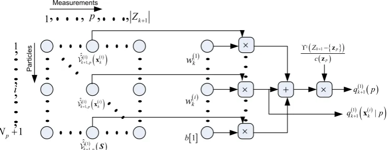
Fig. 2 shows the schematic illustration of the fundamental components of the proposal distributions
and .
As we mentioned earlier, there is no need to apply UT anymore for undetected targets. Consequently, the proposal distribution for sampling is given by
The last step required to obtain detected target three-tuples and undetected target two-tuples is the construction of two proposal distributions and . First, we concentrate on . Let us consider the nth pair of auxiliary variables and which are selected according to (39), as a part of three-tuple
. Hereafter, we drop the index n for notational ease.
The time update for the given pair of auxiliary variables
and pk+1 using unscented transform includes the
following steps
where, according to (8), the function h(.) is defined as
The equations of the measurement update are as follows • • • • • • • • • • • • • • • • • • • • • • • • • • • • • •
( )1
( )
( )1,
ˆˆ i
k+p xk
(1)
( )
( )1 1,ˆˆk+ p xk
( )1 ( ) 1,
ˆˆk+p
S • • • • • • 1 i 1 p N + • • • • • •
1 p Zk+1
• • • • • •
( )1
k w
[ ]1
b
( )i k w × • • • • • • { } ( ) ( )
1 k1 p p
Z c
+
ϒ − z z
( )1 ( ) 1
k
q+ p
,
,
,
( )1
(
( ))
1 i |
k k
q+ x p
,
Measurements Particles,
,
,
,
× × × +Fig. 2. The schematic of how the proposal distributions and are built according to (39) in order to pick up an appropriate existing particle and a new measurement with index p which is likely to be generated from a true target.
( )1 ( ) 1(xi | )
k k
q + p q( )k1+1( )p
(in) k X
(
)
(
)
( )( )
( )(
( ))
1| 11 1 1| ,
x
x p x x x
k k k
N i i i
k i k S k k k
D
b w p f
+ +
+ = +
= +
å
× × (41) (42) (43) (44) (45) (46)
[
]
( )1( )
( ) ( ) ( )1( ) [ ]
1| zp p1 1, x 1, S 1
N i i
k k D i k p k k k p D + p L =
å
=+ ×w ++ ×b1| [ z ] 1| [ z ]
p
p p
N
k k D k k D
D + p L ®®¥D + p L
1| [ zp] k k D
D + p L Dk+1|k[p LD zp]
( )1 ( ) ( )
1
(
x
|
1)
n
i n
k k k
q
+p
+( )1 ( ) 1
(
n1)
k k
q
+p
+( ) ( )2 1
{
x
in}
N n k = ( )
( )
( ) ( )( )
[ ] ( )
( )[ ]
2 1 1 1 . 1 1x x x
x p i k p N i
S i k k k
k k N i
S k i
p w b
q
p w b
d d = + = × + × = × +
å
å
S( ) ( ) ( ) ( )1 ,
1
1 1
{
x
d n,
x
in,
n}
Nn k+ k
p
k+ =( ) ( ) ( )2
,
1 1
{
x
m n,
x
in}
Nn
k+ k =
( )1
(
)
1 1
x | x
k k,
kq
+ +p
( )(
)
2
1
1
x | x
k kk
q
+ +( )1
(
)
1 1 x | xk k,
k
q + + p
( )
x
ink
p
( )kn+1( ) ( ) ( ) ( )1 ,
1
1 1
{
x
d n,
x
in,
n}
N n k+ k
p
k+ = ( )x
i k( ) 2 ( ) ( )
( )
1 0 1| :, , 1, , 1
xi L m x i
p k+-=
å
j=Wj ×c
k+k j i = N + ( ) ( ) ( ) ( ) ( ) ( ) ( ) ( ) ( ) ( ) ( ) ( )(
)
( )( ) ( ) ( )(
)
( )( ) ( ) ( ) ( ) ( ) 21 0 1| 1 1| 1
1| 1|
1|
2
1 0 1|
:, :,
:, 9 :10, , 0, ,2 , 1, , :,
:, 11:12, , 0, ,2 , 1
:,
P x x
+
+
y
L
i c x i i x i i
k j j k k k k k k
x i a i
k k k
i p
k k x i a i
k k k
p L
i m i
k j j k k
W j j
h j j
j L i N
j
h j j
j L i N
W j - - -+ = + + + + + + + -+ = + ¢
é ù é ù
= ×êë - ú êû ë× - úû ìïï
ïï
ï = =
ï = í ïï ïï
ï = = +
ïî = ×
å
c c c c c c å
( )( )
(
)
(
( )( )
)
(
( )(
)
)
( )(
)
(
)
( )( )
(
)
2 21| 1| 1|
1| 1|
:, 1, 3,
3, ,arctan
1,
x i x i x i
k k k k k k
x i k k
x i k k
h j h j h j
h j h j + + + + + é ê = + êë ¢ù æ ö÷ ç ú÷ ç ÷ú ç ÷ ç ÷ú ç ÷÷ çè øúû
c c c
c c ( ) ( )
( )
( ) ( )( )
( ) ( ) ( )( )
( ) ( )( )
( ) 1 1 1 1 2 1| 1 0 1| 1 2 1| 1 0 1| 1 :, :, :, :, y y x y P y y P x y k k k kL c i i
j k k k
j
i i
k k k
L c x i i
j k k k
j
i i
k k k
W j j W j j + + + + -+ + = -+ + -+ + = -+ + é ù
= ×êë - úû
¢
é ù
´êë - úû
é ù
= ×êë - úû
¢
é ù
´êë - úû
å
å
c ( ) ( )(
( ))
( ) ( )(
)
1 1 1 1
1
1 1
1
1 1 1
1 1
x y y y
y y
P
P
x
x
z
y
P
P
P
k k k k k k k
i i i
p
k k k
where zpk+1 is the measurement of the RFS Zk+1 whose index is the auxiliary variable pk+1.
Now, thanks to the by-products of the UT measurement update, we have sufficient means at our disposal to design an efficient proposal distribution . We can generate the nth new sample, , according to the following Gaussian distribution:
where and are given by (46).
In the case of undetected targets, the optimal choice for sampling would be the extended single-state Markov transition density1:
The importance weights are computed to correct the discrepancies due to the usage of the first-stage weights, as it is necessary for the auxiliary particle filter [23]. Note that we should know the true values for functions U0(Z
k+1), U1(Zk+1−{zp}) (for detected targets), and U1(Z
k+1) (for undetected targets) in order to compute the importance weights. In contrast to the predicted estimate, , the update estimate of Dk+1|k[pDLzp] which we will show with can be obtained with new drawn samples instead of the existing particles as follows
where, if we consider new samples whose three-tuples have picked up the pth new measurement, then is the set of the indices of those new samples:
As a result, we can compute the update values (almost true values) of the functions U0(Z
k+1), U1(Zk+1−{zp}), and U1(Zk+1). We replace Dk+1|k[pDLzp] with to obtain ,
,and . The importance weights of
1 Indeed, discussed later on in this section, we will better understand the reason for its optimality after we show that the corresponding importance weights become uniform.
the detected targets are computed as
Remark 1: Consider in (51) so that
equals the Gaussian density . As it is evident, (G5×3. Q3×3.G`)5×5 is not a full rank covariance matrix (two out of five eigenvalues are zero) and therefore the Gaussian
cannot be evaluated at a given . Instead of
we may evaluate the below full rank Gaussian density
The importance weights of undetected targets are computed as
If we consider (43), importance weights of undetected targets is transformed into the following form:
We can see from (54) that the importance weights of undetected targets are uniform. This results in the minimum importance weight variance (equal to zero).
The expected number of targets at the time-step k+1 in the observation area is computed by taking summation of Np elements of the concatenated set . Remark 2: It is not required to perform resampling at the end of each cycle of Auxiliary particle filter family. In fact, resampling step is done before computing importance weights While we are picking up auxiliary variables, we are doing resampling.
The process of applying UT to implement ACPHD is illustrated in the schematic in Fig. 3.
Simulations
We demonstrate the superiority of the proposed Unscented-Auxiliary CPHD (U-ACPHD) filter over the SMC-PHD, (47) (51) (52) (53) (54) (48) (49) (50)
( )1
(
)
1
1 xk | xk,
k
q + + p
( ) ( )1
, 1 1
{xd n N} n k+ =
( )1
(
( ))
(
( ) ( ))
1
x | x
d 1 n,
1x
d 1;
x
n1,
P
n1,
k k k k k k k
q
+ +p
+=
+ + +( )
1 xin
k+ P( )1
n
i k+ ( ) ( )2
, 1 1
{xm n N} n k+ =
( )2
(
( ))
(
( ))
1 x | xm1 n a xm 1|xn , 1, , p 1.
k k k k k
q + + =f + n= N +
1| ˆˆ [k k D zp]
D + p L
1| 1
ˆk k[ D zp], 1, , k
D + p L p= Z +
( ) ( )1
, 1 1
{xd n }N n k+ = ( ) 1
1
{ }
x
n Npn k =+
[
]
(
)
(
)
( )( )
(
( )(
( ))
( )( )
)
( ) ( )(
)
( )(
( ))
( )( )
( ) ( ) ( )( ) [ ]
( )(
)
(
( ))
( )
( ) ( )(
( ) ( ) ( ))
11| 1 1 1
1 | 1 1 1 1 1 1 1 1 1, 1, 1 1, , , 1 1 1 ,
1 1 1
ˆ | , | | , 1 , z z x z x x
x x x
x x
x x
x x
x S
x x x
x | x
p p p i k p n p n N
k k D i D k k
E
i a i
a k
k k k k i
a k
S k i
k
k k
i k
k k
N i i
k p k k k p
i
k p
i
d n d n a
D k k S k
i
d n n
k k k k
D p L p L
f D
p d
q p
q d p
w b
p L p
q p d + + = + + + + + + + + + = + + + + + + = × × ´ × × ´ × + × =
é × ×
ê
´ ê
ê ë
å ò
å
T ( ) ( )
(
)
( )( )
( ) 1, , 1 1 1, | , x x x k p n n n i d na k k
i k p k
f + Î + + ê ù ú ´ ú ú úû
å
T 1,k+ p
T
1|
ˆk k[ D zp]
D + p L ¡ˆ (0 Zk+1)
1 1
ˆ (Zk+ { })zp
¡ - ¡ˆ (1 Zk+1)
()
(
( ) ( ) ( ))
( ) ( )(
)
( )(
( ))
( )( )
( ){ }
(
)
(
)
( ) ( )(
)
( )( )
( )
( ) ( )(
( ) ( ) ( ))
( ){
}
1 1 11 , , ,
1 1 1 1 1 1
1 1 , 1 0 1 | 1 1 ,
1 1 1
1 ,
ˆ
1 |
ˆ
, 1, ,
, ,
, 1, , .
z
x ,x x x
z x x z x x x x n n pk n n k n k n n n i
d n n d n d n
D
k k k k k k
k p i
d n a k k k p i i a a
S k k k k i
d n n
k k k k
n p
w p p L
N Z f Z c p D n N q p i N + + + + + + + + + + + + + + = × × ¡ -´ × × ¡ × ´ = Î ( ) xin S
k ¹ ( ) ( ) ( ) ( )
, ,
1 1
(xd n |xin ) (xd n |xin )
a
k k k k
f + =f +
( ) ( ) ( )
, 1
(xd n; (xin (5)) xin,G Q G) k+ F k × k × × ¢
N
( ) ( )
, 1
(xd n |xin )
k k
f +
( )
, 1
x
d nk+ (x ,( )1 |x( ))
n i d n k k f + ( )
(
(
( )( ))
( ))
(
1)
3 1
1 5 ; , .
G G G xd xn xn 0 Q
k F k k
-´ + ¢× × ¢× - × N ( )
(
( ) ( ))
(
)
( )(
)
(
)
( ) ( )(
)
( )
( )( )
( ) ( )(
( ) ( ))
( ){
}
1 1 2 ,1 1 2 0
1 , 1 | 2 , 1 1 2
ˆ
1
ˆ
|
.
,
1, ,
,
1, ,
x
,x
x
x
x
x
x
x
n
n n n
n
D k
i m n
k k k
k
i i i
m n a a
a
S
k k k k k k
i m n
k k k
n p
p
Z
w
N
Z
f
p
D
q
n
N
i
N
+ + + + + + +
-
¡
=
×
¡
×
×
´
=
Î
( )
(
( ) ( ))
( )[ ]
( )
(
)
(
(
)
)
( )
{
}
2 , 1
1 1 0
2 1 1 1 2
1
ˆ
ˆ
1
1, ,
,
1, ,
.
x
,x
p n N i S k im n i
k k k
k
D k
n p
p w
b
w
Z
N
p
Z
n
N
i
N
= + + + +
×
+
=
¡
×
-
¡
=
Î
å
( )1 ( )1 ( )2 ( )2
1 1
1 1
{ (.,.,.)}N { (.,.)}N
n m
k k
w + = w + =
( )
{
}
1,
:
n1.
k p k
SMC-CPHD and Unscented-Auxiliary PHD (U-APHD) filter by simulation results. The implementation method for the SMC-PHD and SMC-CPHD filter are described in [14,15]. We follow the same procedure described for the U-ACPHD filter in order to implement the U-APHD filter expect that the update and correction steps of the U-APHD filter is modified according to the PHD recursion [17].
In our simulations, we confine observations to a square region with sides equal to 1km while the sensor is located in The simulation scenario parameters are denoted in Table 1. For the SMC-PHD and SMC-CPHD filter, we set the numbers of particles assigned to sample from the intensity function of newly born and persistent targets to 500 and 2500 respectively, which are fixed regardless of the expected number of targets. For the birth intensity function, we set mb=[500,0,500,0,0]` and Qb=diag(152,52,152,52,0.12).
There are 5 targets appearing and disappearing during the simulation time of 90 time-steps (nearly 100 time-steps), so the predicted number of newly born targets b[1]=gb is 5/100. The spatial distribution c(z) is uniform over range and bearing domain [0,1000]×[0,p/2] and average number of clutter points l equals 10. We set g and b−a2 to 2 and 0 respectively in (34).
UT prediction step
UT update step ( )1 ( )
1 ,
k
w+ ⋅ ⋅ ⋅,
( )2 ( ) 1 k
w+ ⋅ ⋅,
( ) ( ) ( )
, 1, , 1
i i k k i
k p
w i N
= +
x P
UT sigma points
( )
,
a i k
c
( )1 ( )
1,
ˆˆ ( i) k+ pxk
predicted estimate
1|
ˆˆ
p
k k D
D+ p Lz
( )1 ( )
1 k|
k
q+ x p construct
1)( )
1 k
q+ p
{ }
( )
1 1
ˆˆ Zk+ p
ϒ − z
( ) ( )1
1
i k
i k
− +
− +
x P
( ) ( )1
1
i k
i k
+
+
x P
next time-step ( )1
(
( ))
1 1 k | i,
k k
q+ x+ x p
update estimate
1|
ˆ
p
k k D
D+ p Lz
( )
{ }
(
1)
1 1
ˆ n
k
k p
Z +
+
ϒ − z
( )
1 1
ˆ Zk+
ϒ
Importance weights
( )
0 1
ˆ Zk+
ϒ
( ) ( ) ( )
{
}
( )1,
1 1
1
, in, N
d n n
k k k
n
p + +
=
x x
Fig. 3. The schematic of how UT can be used to implement ACPHD filter and construct proposal distributions as well as computing importance weights.
Parameter Value
T 1 s
se 0.1
sw p/180 rad/s
sq 0.5×p/180 rad
sr 1 m
pD 0.95
ps 0.99
N(1) 2500
N(2) 500
Simulation length 90 time-steps
Table 1. Simulation Scenario Parameters
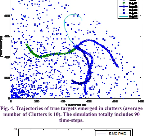
Fig. 4. Trajectories of true targets emerged in clutters (average number of Clutters is 10). The simulation totally includes 90
time-steps.
Fig. 5. The OSPA distance for different filters versus simulation time-step, averaged over 100 Monte Carlo runs. An average
Our scenario of interest, consisting of five targets whose trajectories are merged into clutter, is shown in Fig. 4. In addition, the related initial states and appearance and disappearance time-steps of targets used in the simulation scenario are all illustrated in Table 2.
The true number of targets at each time-step can be obtained from the target appearance and disappearance times in Table 2. We computed the OSPA, cardinality, and localization distance between the set of target state position estimates and true target positions at each time-step in order to compare performance of the four aforementioned tracking algorithms (see [25] for more details about these distances). Each distance is obtained by averaging over 100 Monte Carlo runs. Two parameters of the OSPA distance, the OSPA order (r) and the OSPA cut-off (c) are set to 2 and 150 m respectively. The SMC-PHD, SMC-CPHD, U-APHD, and U-ACPHD filter approximates intensity function with particle samples and do not explicitly provide any state estimate.
We apply the natural clustering methods for extracting target states from the sample-based approximated U-APHD and U-ACPHD filter. The method is valid thanks to the principle of auxiliary variables and described in [16,17].
However, it would not work for the case of the SMC-PHD and SMC-CPHD filters and so we apply the k-means clustering function in MATLAB, and set its parameters as follows: ‘distance’=’city’ and ‘replicates’=’5’.
As shown in Fig. 5, the OSPA distance is getting larger when we see a growth of the number of targets much like what happens for the period started from the time-step 21 up to the time-step 70, common for all filters. This is due to using fixed number of particles regardless of the expected number of targets. As a consequence of this strategy, the number of particles assigned to each tracked target decreases and this leads to poor estimation performance.
Apart from this fact, as shown in Figs. 5-7, the U-ACPHD outperforms in terms of the localization accuracy and the cardinality estimation because the U-ACPHD filter uses two auxiliary variables to utilize the most current information to improve both the cardinality density and intensity function. Of the other methods tested, the U-APHD filter offers the next best performance, and that is because it applies auxiliary variables to only improve the estimation of intensity function.
We can see that the SMC-PHD filter has the worst results in cardinality estimation and localization performance compared to other filters.
Indeed, as pointed out in [5], the value of the expected number of target for the SMC-PHD filter is very unstable in the presence of misdetection and there is a high probability to lose a confirmed track. This justifies its higher OSPA, cardinality and localization distances for the last time-steps. In order to assess the impact of average number of clutter points on estimation of intensity function, we compute the OSPA, cardinality, and localization distance over the 100 Monte Carlo runs, for various values of l. These distances are then averaged over the entire period of simulation time (90 time-steps). The results are represented in Table 3. According to the Table 3, the U-ACPHD filter again outperforms the rest of filters in terms of all average distances for all tested values of l. Its robustness and accuracy in different environments (especially in high-clutter environments) justify the complexity involved in the implementation of the U-ACPHD filter. To our surprise, the SMC-PHD filter has the second best performance. One part of the reason for this behavior is traced to the fact that the CPHD filter is more robust than the PHD filter from increase in the average clutter rate especially near the origin.
Near the origin, because of the higher incidence of false alarms, false tracks can be considered as candidates of targets with very low probability of detection. However, the SMC-PHD is not good to keep track of targets with low probability of detection and seems to be less vulnerable to higher clutter ratings. The reason for the superiority of the SMC-PHD filter over the U-APHD filter in scenarios with high clutter lies with the usage of auxiliary variables which improves the localization estimation accuracy for true tracks and leads to low localization distances. As a result, the APHD filter accounts for false tracks and tries to prolong them. The consequences of these tendencies are little localization distance versus high cardinality distance. The solution to these vulnerabilities is to enjoy the benefits of synergy obtained by combination of updating cardinality distribution as well as using auxiliary variables to estimate the intensity function. This is what exactly the U-ACPHD filter is doing, which yields a real compromise between cardinality and localization distance in harsh environments , as it is evident in Table 3.
Fig. 6. The localization distance averaged over 100 Monte Carlo runs. An average number of Clutter points is 10. Compared to the auxiliary particle based filters, both the SMC
filters have failed in performance of localization estimation fo time-steps in which all the targets are present.
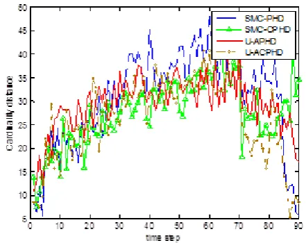
Fig. 7. The cardinality distance averaged over 100 Monte Carlo runs. An average number of Clutter points is 10. Apart
The reason for the superiority of the SMC-PHD filter o