TWO APPROACHES ON CARRIER FREQUENCY OFFSET ESTIMATION IN MIMO OFDM SYSTEMS

Printed in The Islamic Republic of Iran, 2014 © Shiraz University

TWO APPROACHES ON CARRIER FREQUENCY OFFSET

ESTIMATION IN MIMO OFDM SYSTEMS*

M. SALEHPOUR AND M. R. TABAN**

Dept. of Electrical and Computer Engineering, Yazd University, Yazd, P.O.Box: 89195-741, I. R. of Iran Email: mrtaban@yazd.ac.ir

Abstract– We consider the problem of joint carrier frequency offset and channel estimation

between transmitter and receiver in a frequency-selective channel MIMO-OFDM system. Recently two high performance estimators based on the expectation-maximization (EM) algorithm have been proposed. The main drawback of the maximum likelihood base algorithms, like EM algorithm, is the high computational complexity. In this paper, we propose an extended Kalman filter based estimator, which has higher performance than that of EM algorithm, while its computational complexity is lower. In addition, the Particle Swarm Optimization (PSO) algorithm is used for joint ML estimation of carrier frequency offset and channel parameters for the general model. The proposed method has a lower computational complexity than that of traditional search methods. Simulation results in comparison with Cramer-Rao bound show that the proposed algorithms outperform the EM in all ranges of signal-to-noise ratio for both channel and frequency offset estimations. Also, among them, the PSO algorithm is superior.

Keywords– Carrier frequency offset (CFO), estimation, MIMO-OFDM, extended Kalman filter (EKF), particle

swarm optimization (PSO)

1. INTRODUCTION

The combination of multiple-input multiple-output (MIMO) wireless technology with orthogonal frequency division multiplexing (MIMO-OFDM) is a remedial solution for next generation wireless local area networks (WLANs), wireless metropolitan area networks (WMANs), and fourth-generation mobile cellular wireless systems. Since OFDM offers the possibility for high data rates at low decoding complexity, it has been widely adopted by many standards (e.g., IEEE802.11a, IEEE802.11g in the U.S., and digital audio/video broadcasting (DAB/DVB), HiperLAN/2 in Europe) [1, 2], although OFDM is a promising technique, especially when we combine it with spatial diversity techniques, i.e., MIMO systems in more general case, its high sensitivity to carrier frequency offset (CFO) due a difference between the carrier frequencies of the local oscillators at the transmitter and the receiver, produces inter carrier interferences (ICI) and causes desired signal attenuation, and as such introduces a huge performance loss.

Whereas OFDM is robust to the multipath delay, in order to achieve high-quality transmission [3] and avoid phase and amplitude distortion due to coherent detection and decoding in fading channel, the estimation of channel parameters and compensation is necessary in addition to the frequency offset estimation. Joint estimation of CFO and channel impulse response (CIR) parameters leads to particularly complex problems because of the number of unknowns [4]. A number of approaches have dealt with the CFO and channel estimation in a single-input single-output (SISO) OFDM setup in literature [5, 6]. Although the CFO estimation is a well studied problem in the SISO systems, it is relatively novel for the

MIMO-OFDM systems. In SISO OFDM, some methods rely on training blocks [7, 8], while others just take advantage of standard transmission format; e.g., exploit the presence of null sub-carriers and save the transmission bandwidth by blind estimation [9, 10]. In order to obtain the maximum-likelihood (ML) estimation of CFO, the prohibitive computational complexity is required [11]. Saemi et al. in [12, 13] have proposed a new algorithm for time-frequency synchronization joint with the channel identification in MIMO-OFDM systems. The high complexity is one drawback of this method. Salari et al. in [14] have proposed a ML solution in an iterative manner; e.g., expectation-maximization (EM) algorithm [15]. Their CFO estimator first provides a CIR estimate in the expectation (E)-step and then estimates the CFO in the maximization step (M)-step. Because of the estimator complexity, they have also proposed a simpler estimator with a decrease in performance.

The Extended Kalman Filter (EKF) has been widely used for estimation in non-linear systems [16]. In this paper, we propose a CFO estimator based on the EKF whose complexity is less than that of ML estimator, although its performance is better. Moreover, according to the Particle Swarm Optimization (PSO) theory, a joint ML estimation algorithm of CFO and channel for the general model is proposed. The advantages of the proposed algorithm are that it is simple in conception, easy to implement, and efficient in computation. The PSO-based estimation algorithm has a lower computational complexity than that of traditional search methods. This makes the computational efficiency of the mentioned method higher.

The rest of the paper is organized as follows: The next section contains an introduction to MIMO-OFDM system model which experiences carrier frequency offset. Section III briefly explains the ML, EM, and proposed algorithms. This paper ends with the simulation results and conclusion in section IV and V.

2. MIMO-OFDM SYSTEM MODEL

A discrete-time FFT/IFFT-based N_t´N_r MIMO-OFDM system is considered and its typical structure as a block diagram is shown in Fig.1. The time-domain complex baseband samples ì üï ïï ï_{í ý}

j

,

j

1,...,

N

t

ï ï ï ï

î þ

s

=

with

c

N

subcarriers are generated by taking N_c-point inverse fast Fourier transform IFFT

c

N

ì ü

ï ï

ï ï

í ý

ï ï

ï ï

î þ of a block of subcarrier symbols

{ }

X_j . Then we construct

{ }

u

_j ,j=1,...,N_c+N_g by adding a cyclic prefix with

length N_g preceding each symbol, which should be longer than the CIR length (L), so that there will be no inter-symbol interference (ISI). Then the baseband signal is up-converted to the radio frequency (RF) fc

after parallel-to-serial (P/S) conversion, and transmitted through the

N

_t transmit antennas. The channel is a Rayleigh frequency-selective fading which is described by complex Gaussian matrix elements. Also, it is assumed that the fading process remains static during each OFDM word (one time slot) and varies from one OFDM block to another. The fading processes associated with different transmitter-receiver antenna pairs are uncorrelated. At each receive antenna, a superposition of faded signal plus noise is received. Received signals are down-converted to baseband with the local oscillators centered at

f

ˆ

_c. The samples at the

i

th receive antenna filter can be written as [14]

2 exp j

1 ,

1 0

( ) ( ). ( ) ( ), 1,2,...,

c t k N

N L

i i j j i r

j l

r k ï_íïìï pe ïïü_ýï h l u k l v k i N

ï ï ï ï ï ï î þ

-= -=

=

å å

- + = (1)

Fig. 1. Transmitter-receiver structure of a Nt× Nr MIMO-OFDM system [14]

( ) j

u k is the sample of u_j after P/S in time k, ε is the CFO normalized to the subcarrier spacing 1 /T and

( )

i

v k

is the channel noise sample that is an additive white complex Gaussian noise with zero mean and variance 2

i v

s . After serial-to-parallel (S/P) conversion and removing the cyclic prefix, we will reach

y

_i in the

i

th receiver as

2

exp j _,

1

( ). . , 1,2,...,

g c t N N N

i j i j i r

j i N pe _e ì ü ï ï ï ï ï ï í ý ï ï ï ï ï ï

î þ ₌

=

å

+ =

y F A h v    

where

 ( ) 1,exp j2 ,.. exp j., 2 ( 1) ,

c c _N

c c

c _N

N N N

diag pe pe

e

´

ì ü ì ü

ï ï ï ï

ï ï ï ï

ï ï ï ï

í ý í ý

æ _ö÷

ç _÷

ç - ÷

ç ÷

ç _÷÷

çè îïïï ïïþï ïîïï ïïïþø =

F    

, c , 1 , 1 ,

j_{a b} s a bj _N a Nc b L

æ _ö÷ é ù ç_{ç ÷} ÷ ê ú ç_ç ÷

ê ú ÷

ëA û = _çè - ÷_ø £ £ £ £  

and _{i j, ê}éê

h

_{i j,} (0)

,...,

h

_{i j,} (L-1)úù_úT

, 1

j

N

_t

, 1

j

N

_r

ë û

=

£ £

£ £

h

describes the L order realization of the

channel between the jth transmitter and the

i

th receiver. The random vectors h_{i j,} are assumed to be independent with zero mean complex Gaussian distribution. s_j( )p denotes the pth entry of s_j for

1

£ £

p N

_c and

k

q

denotes the modulo-K of q that is located in the interval _ëéê

0,

K

-

1

ù_ûú, indeed A_j is in the form (5) to implement the convolution operator.

(0) ( 1) ( 1)

(1) (0) ( 2)

( 1) ( 2) ( )

c c

c

c c c

N N L

N L

N N N L

j j j

j j j

j

j j j

s

s

s

s

s

s

s

s

s

é _{- - +} ù

ê ú

ê _{- +} ú

ê ú

ê ú

ê ú

ê ú

ê _{- - -} ú

The vector v_i containing the channel noise samples

v

_i( )k , is complex Gaussian with zero mean and covariance matrix 2

i v

s I We can simplify the input-output equation (2) by rewriting it in matrix form as

( ). ( ). , 1,...,

i= e e i+ i i= Nr

y F A h v    where

( )

1

. , ... ,

2 2

exp j exp j

t c t

g g N

N N L

N N

Kpe Kpe

e _êêé ïïïì üïïï ïïïì ïïïü ùú_ú

ê ú

ê ú

ë

í ý í ý

ï ï ï ï

ï ï ï ï

ï ï ï ï

î þ î þ _{û ´}

=

A A A    

,1

,

,2

, ...,

, _{t . 1}

t T

T T T

i _{i i i N}

N L

é ù

ê ú

ê ú

ê ú

ë û ´

=

h

h

h

h

  

Here, the channel and noise are assumed to be statistically independent.

3. JOINT CFO AND CIR ESTIMATION

a) ML estimation and EM algorithm

The transmission model has two unknown parameters: the normalized CFO, ε, and the coefficients of CIR, i

h

(

i

=

1,...,

N

_r). Based on the signal model in (6), the ML estimation of parameters {e,h_i} is given by maximizing the likelihood function that is equivalent to minimizing the cost function shown below:

2

, ₂

1 1

min r ( ) ( )

i

i N

i i

i v

e _s e e

ì ü ï ï ï ï ï ï ï ï ï ï í ý ï ï ï ï ï ï ï ï ï ï

î = þ

-å

h y F A h   

First, assuming the CFO to be fixed and because of independence between

h

_is the ML estimate of

h

_i is obtained as

( ) ( ) 1

ˆ _{( ) ( ) , 1,...,}

r

H H H

i =_èçæçç e e_÷÷ö÷_ø÷ e e i i N

-=

h A A A F y    

Then substituting

h

ˆ

_i into (9) and after some manipulation, we obtain the estimation of e as

2 1

2 1

1

ˆ argmax r ( ) ( ) ( ) ( ) ( )

i N

H H H

i

i v

e

e e e e e e

s

ì ü

ï ï

ï ï

ï ï

ï æ ö ï

ï ï

ï ç ÷_÷ ï

í ç_{ç ÷÷} ý

ï è ø ï

ï ï ï ï ï ï ï ï ï ï î þ -=

=

å

A A A A F y   

The above ML estimation method of CFO requires a huge computational search over the trail values of CFO. Although the accuracy of ML estimation is high, this computational complexity makes a serious challenge in the practical applications.

To circumvent this problem, Salari et al. in [14] have used the EM algorithm. In [14], the CIR parameters are obtained in the expectation step and the CFO is estimated in maximization step. They have also formed a computationally simpler CFO estimator with a slight loss. In this paper, we consider the first estimator of [14] as EM algorithm which is called EM.

b) Extended Kalman filter

1 1

(

)

n

=

f

n-

+

n

-x

x

w



( )

n

= G

n

+

n

y

x

v



where

x

_n,

y

_n,

w

_n-1, and

v

_n are the state vector, observation vector, state noise and measurement noise respectively, these two stages are presented by the following equations:

Time Update Equations:

| 1 1| 1

ˆ

_{n n}

f

æç_ç

ˆ

_{n n} ö÷_÷÷

ç ÷

çè ø

-

=

-x

x



1 1

| 1 n 1| 1 T 1 n

n n-

=

- n- -n n-

+

-P

F

P

F

Q

  

Measurement Update Equations:

| | 1 | 1

ˆ_{n n} ˆ_{n n n n}çæ_çç æ_ççˆ_{n n ÷÷}ö÷÷_÷÷÷ö

ç ÷

ç

ç è ø÷

çè ø

-

-= + - G

x x K y x   

1

| 1 T | 1 T

n n n n n n n n n

æ _ö÷ ç _÷ ç ÷ ç ÷ çè ø -- -= +

K P H H P H R   

| ( n n) | 1

n n= - n n

-P I K H P 

where

ˆ

x

_{n n| -1} and P_{n n| -1} are the predicted state and estimate covariance respectively,

x

ˆ

_{n n|} and P_{n n|}

are the updated state and estimate covariance from the data until time n respectively, and

ˆ_{n n|}

n=_¶¶f

x

F x

and

ˆ_{n n| 1}

n -¶G =_¶ x H

x . Also,

K

n is the Kalman gain,

R

n and

Q

n are the measurement and state noise

covariance matrices and n is the number of EKF updating step. When

R

_n and

Q

_n are unknown, they can be ML estimated during execution of the EKF steps from the equations below:

1

1 n _{ˆ ˆH}

n l l

l n M M

=

-=

å

R v v 

1

1 n _{ˆ ˆH}

n _{l l}

l n M M

=

-=

å

Q w w 

where

ˆ

_{l l}

æ

ç

ç

ˆ

_{l l| 1-}

ö÷

÷

÷

è

ø

=

- G

v

y

x

and

ˆ

_l

ˆ

_{l l|}

f

æ

ç

ç

ˆ

_{l- -1| 1l}

ö÷

÷

÷

è

ø

=

-w

x

x

, and M is the number of estimated

noise vectors in the ML estimation.

The time update equations are responsible for projecting forward (in time) the current state and error covariance estimates to obtain the apriori estimates for the time step. The measurement update equations are responsible for the feedback, i.e., for incorporating a new data into apriori estimate to obtain an improved aposteriori estimate. The time update equations can also be thought of as predictor equations, while the measurement update equations can be thought of as corrector equations.

e_n+1=e_n+w_n

where the state noise

w

_n is assumed to be an additive white complex Gaussian noise with zero mean and unknown variance 2

n w

s . Notice that in this model, state variable

x

_n and state noise

w

_n-1 are scalar (denoted as

e

_n and

w

_n respectively). The measurement equation (observation vector) can be reformulated as



y

_n

= G

( )

e

_n

+

v

_n where the nonlinear function



 

.

of the state variable

e

_n is defined as

G

( )

e

_n

=

F

( ) (ˆ)

e

_n

A h

e

ˆ

_i. Consider that

A

(ˆ)

e

has been computed by (7) for eˆ=eˆ_{n n| -1} and

h

_i has already been estimated by an ML

solution as ˆ_i êé (ˆ)eH (ˆ)eùú 1 (ˆ)eH (ˆ)eH _i

ê ú

ë û

-=

h A A A F y , like the E-step of the EM algorithm in [14].

Since the observation equation is a nonlinear function of the CFO, an EKF-based algorithm is used to estimate the CFO. Let eˆ_{n n| -1} be our apriori state estimation at step n, given knowledge of the process

prior to the step n, ˆe_{n n|} be our aposteriori state estimation at step n given data

y

_n and P_{n n| -1} and

|

n n

P are apriori and aposteriori error estimation covariance respectively.

c) Proposed CFO estimation algorithm

In the proposed EKF algorithm,

N

_r data streams (each stream contains

N

_c samples) are used to estimate the CFO. Each data stream per receive antenna is consecutively used for one updating step of EKF procedure; in other words, here, the number of EKF updating step n is the number of receive antenna. Since the number of receivers is not a lot, to improve the EKF algorithm, we propose an iterative procedure. In this method, after updating the CFO during

N

_r updating steps using data from the first receive antenna to the last receive antenna, the estimated CFO of EKF is fed back to the EKF algorithm as an initial CFO (eˆ₁₀), and the EKF algorithm is again repeated by the new initial value. In the new iteration; P_1|0 is also substituted from the previous iteration. Although the

N

_r´

N

_c data symbols are the same in the different iterations,

e

ˆ

and P improve during each iteration because of passing the transient state. Due to the iterative nature of this algorithm, we call it Iterative Extended Kalman Filter (IEKF). This iterative procedure can be continued until the rational mean square error (MSE) is achieved.

d) Particle swarm optimization algorithm

Particle Swarm Optimization, inspired by the social behavior of swarms of birds and fish schools, is a high performance optimizer first presented by Eberhart and Kennedy [17]. Compared to the conventional optimization techniques such as the Genetic Algorithms (GA), the PSO benefits from its algorithmic simplicity and robustness. The PSO exploits a swarm of particles which seek the promising regions of the D-dimension search space with adaptable velocity. Each particle changes its position based on its encountered best position and the best position attained by all particles.

Consider m particles with position and velocity vectors as

x

_i and

v

_i,i=1,2,...,mrespectively. The equations of updating the velocity and position in the PSO are stated by (23) and (24) as

( 1) ( ) ( ) ( ) ( ) ( ) ( )

1 1 2 2

,k k ,k ,k ,k k ,k

i j i j i j i j j i j

v

w v

c r pbest

_çççæ

x

_÷÷÷ö_÷

c r gbest

æ_ççç

x

÷_÷÷ö_÷

ç ÷ ç ÷

ç ç

è ø è ø

+

=

+

-

+

-

_{  }

(

1)

( )

(

1),

1,..., ,

1,...,

,

k

,

k

,

k

i

m j

J

i j

i j

i j

where

-

v

i j

( )

,

k is the _jth _{component of velocity vector of particle i at iteration k.}

-

v

i j

(

,

k+1

)

is the _jth _{component of modified velocity vector of particle i at next iteration k+1.}

-

x

i j

( )

,

k

is the _jth _{component of position vector of particle i at iteration k.}

-

x

i j

(

,

k

+

1)

is the _jth _{component of the modified position of particle i at next iteration k+1.}

- r r_{1 2}, are random numbers between 0 and 1 (representing the random movement of each particle).

- pbest_{i j}( )_,k is the _jth_{component of} ( )k i

pbest

which is the best position found by the particle i at iteration k.

- gbest( )_jk is the _jth _{component of}

gbest

( )k _{which is the best position found by the particle} swarm separately at iteration k.

- c c₁, ₂ are positive constants (weigh the influence of individual and social learning, respectively).

- w( )k is inertia weight at iteration k.

The inertia weight factor w balances the ability of exploration (global search) and exploitation (local search). In general, the large value of w is prone to global region hunting and the small value of w helps local region probing. Linearly decreasing inertia weights were recommended in [18] and PSO with decreasing inertia weights has better performance. The mentioned inertia weight is as follows

( ) max min

max max

max

,

1,2,...,

k

w

w

w

k k

k

k

w

=

-

-

´

=

  

where

w

_min and

w

_max represent the range of inertia weight and

k

_max is the maximum iteration number.

In general, the PSO algorithm can be described as follows:

1) Initialize each particle i of the population by randomly selecting values for its location

x

( )_ik and velocity ( )k

i

v

vectors.

2) Calculate the fitness value of each particle. If the current fitness value for the particle is greater than the best fitness value found for the particle so far, then

pbest

( )_ik is updated.

3) Determine the location of the particle with the highest fitness and update

gbest

( )k _{if necessary.} 4) For each particle, calculate the velocity according to the equation (23).

5) Update the position of each particle according to the equation (24).

6) Repeat steps 2-5 until reaching the termination condition (number of iterations or precision).

Before employing the PSO method to solve the CFO estimation, two definitions must be made as follows: 1) Representationof the particle. The particle is the CFO (ε) in our problem, 2) Determination of the fitness function. According to (11), the fitness function is

2

1 2

1

1 _{( ) ( ) ( ) ( ) ( )}

r

i

N

H H H

i

i v

FIT e e e e e

s

æ _ö÷

ç _÷

ç _÷

çè ø

-=

=

å

A A A A F y    

4. SIMULATION RESULTS

In this section, we present the results of simulations to demonstrate the effectiveness of the proposed schemes. The system parameters are presented in Table 1 which are held constant throughout the simulations. The data symbols are complex independent and identically distributed from 4-QAM constellation with

s

2

x

=1. The signal-to-noise-ratio (SNR) is defined as

SNR

=

E

_x/

s

_v2 where

E

_x is the total transmitted signal energy and

s

_v2 is the variance of channel noise corresponding to each receiver. Given the parameters in Table 1, the simulations have been executed with 1000 Monte Carlo iterations. We have also used

ˆ

e

_1|0=0 and P_1|0

=

I for IEKF initialization and assumed known

0

=

s

v

2 N_c´N_c

R

I

equal to noise covariance for each receive antenna.

Table 1. System settings in simulations

Number of carriers 128

Channel power delay profile (PDP) [0.55,0.24,0.11,0.04,0.02] Guard time (Cyclic Prefix) 5 symbol period

Modulation 4-QAM

In the simulation of the PSO algorithm

c

₁ and

c

₂ are set to 1.49 [19],

w

_max (w in start) and

w

_min (w in end) are 0.64 and 0.4,

k

_max and swarm size (m) are equal to 20 and 16 respectively.

For performance evaluation, the MSE of the normalized CFO estimation i.e.

E

æçç_ç

e e

ˆ

2ö÷÷_÷÷ ç _÷÷

çè

-

ø is applied.

We also use the MSE as E ˆ2

æ _ö÷

ç _÷

ç ÷

ç ÷

ç ÷

ç ÷

ç ÷÷ çè ø

-h -h for channel estimation evaluation, where ₁, ₂,...,

r

T T

N

T T

é ù

ê ú

ê ú

ë û

=

h h h h .

a) Performance evaluation of the proposed algorithms

We first consider four 2×2, 3×3, 4×4 and 6×6 MIMO-OFDM systems in the simulation and the CFO is set as

e

=

0.1

. Fig. 2 and Fig. 3 depict the MSE of CFO estimation versus SNR for the IEKF and PSO methods respectively. Here, SNR is varied from 0 to 30 dB over a frequency-selective fading channel. From Fig. 2 and Fig. 3, it can be observed that the performance of both algorithms is satisfactory even in low SNR and small number of antennas. Also, as predicted, by increasing SNR or the number of transmit-receive antennas, their performance improves.

Fig. 3. MSE of CFO estimation by PSO versus SNR for different number of transmit-receive antennas in  = 0.1

Then, for performance comparison, we consider a 2×2 MIMO-OFDM system and set the CFO as

0.06

e

=

. In Fig. 4, the MSE of CFO versus SNR for IEKF and PSO methods is compared to that of EM method and Cramer Rao Bound (CRB) [14. Eq. (27)]. It can be found that while the performance of the IEKF algorithm is better than that of EM, the PSO outperforms both of them and is closer to the CRB. The main point is the huge complexity reduction in the IEKF algorithm compared to the EM algorithm. Furthermore, it is noticeable that the performance of the IEKF algorithm and PSO method is more improved when the SNR increases.

Fig. 4. Comparison between the accuracy of the proposed CFO estimators with that of EM method and CRB in  = 0.06

Table 2. Average execution times of the proposed methods in comparison with the EM method Estimation Method Execution Time (sec)

EM 3.34 IEKF 0.09 PSO 0.57

For evaluating the performance of the proposed algorithms in various values of real CFO, we present the MSE of CFO estimation curves versus the real CFO (

e

). Figures 5 and 6 show these curves for two different values of SNR for the IEKF and PSO method respectively.

Fig. 5. MSE of CFO estimation by IEKF versus real CFO (e) for two different values of SNR

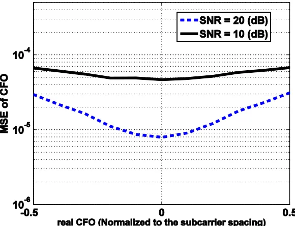
Fig. 6. MSE of CFO estimation by PSO versus real CFO (e) for two different values of SNR

figures, the previous results according to some selected values of CFO can be generalized to all values of CFO. However, the MSE of CFO estimation in the IEKF method becomes less for smaller real CFO. It is clear that the acquisition range of the proposed algorithms is at least equal to one subcarrier spacing.

b) Performance of IEKF for different number of iteration

The number of iteration is an important parameter in the IEKF algorithm. In Fig. 7, we evaluate the effect of number of iteration in the IEKF algorithm. The MSE performance has been obtained for a 2×2 MIMO-OFDM system and the CFO has been fixed on 0.1. It is obvious that increasing the number of iterations improves the performance of the algorithm; nonetheless, what is significant is that with more than 10 iterations, the perfect performance is almost provided. Thus, in the related simulations, we have set the IEKF iterations to 10.

Fig. 7. MSE of CFO estimation by IEKF versus the number of iterations for two different values of SNR

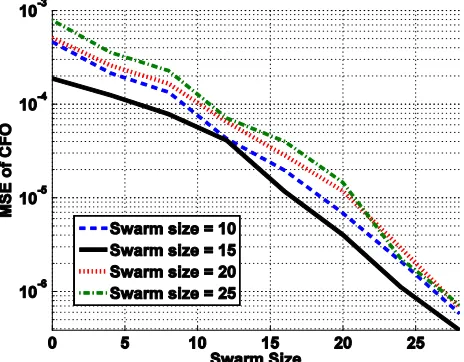
c) Investigating on the selection of parameters of PSO algorithm

In Figs. 8, 9, and 10, we illustrate the effect of inertia weight (w), maximum iteration number æç_ç

k

_maxö÷_÷

÷ ç ÷

çè ø and swarm size (m) in the performance of PSO algorithm respectively. The MSE performance has been obtained for a 2×2 MIMO-OFDM system with CFO equal to 0.2. As shown in Fig. 8, changing the interval of inertia weight has little effect on the performance of PSO algorithm. Also, regarding Figs. 9 and 10, it is concluded that a choice larger than 10 for

k

_max and equal to 15 for the swarm size is suitable for getting an appropriate performance.

d) Performance of estimation of CIR

Fig. 8. Investigation of the effect of inertia weight in PSO algorithm by using various interval (wend,wstart) in ε 0.2

Fig. 9. Investigation of the effect of iteration number in PSO algorithm

Fig. 11. The MSE performance of proposed methods in channel estimation in comparison with that of EM method and ideal case in ε 0.06

5. CONCLUSION

In this paper, we proposed a novel iterative carrier frequency offset estimation algorithm based on the EKF algorithm and multi-antenna channel ML estimation for MIMO-OFDM systems. In the proposed scheme, we implement the EKF updating steps on the number of receive antennas and, after each cycle, the last estimated CFO of EKF is fed back to the estimator iteratively. The PSO algorithm was also used for CFO ML estimation. The proposed algorithms not only outperform the EM algorithm, but also have much lower computational complexity. The performance of our estimators was investigated by computer simulations and benchmarked with CRB. Simulation results show that the accuracy of the proposed algorithms is close to the CRB.

NOMENCLATURE

MIMO multiple-input multiple-output

OFDM orthogonal frequency division multiplexing WLANs wireless local area networks

WMANs wireless metropolitan area networks CFO carrier frequency offset

ICI inter-carrier interference CIR channel impulse response SISO single-input single-output

ML maximum-likelihood

EM expectation-maximization EKF extended Kalman filter PSO particle swarm optimization FFT fast Fourier-transform IFFT inverse fast Fourier-transform ISI inter-symbol interference RF radio frequency

P/S parallel-to-serial S/P serial –to-parallel

IEKF iterative extended Kalman filter MSE mean square error

REFERENCES

1. Negi, R. & Cioffi, J. (1998). Pilot tone selection for channel estimation in a mobile OFDM system, IEEE Trans. Consum. Electron, Vol. 44, pp. 1122–1128.

2. Wang, Z. & Giannakis, G. B. (2000). Wireless multicarrier communications: Where Fourier meets Shannon. IEEE Signal Process. Mag., Vol. 47, pp. 29–48.

3. Salari, S., Ahmadian, M., Ardebilipour, M., Cances, J. P. & Meghdadi, V. (2008). EM-based turbo receiver design for LDPC coded MIMO–OFDM systems with carrier-frequency offset. IET Commun., Vol. 2, pp. 107– 112.

4. Ma, X., Oh, M.K., Ginnakis, G. B. & Park, D. J. (2005). Hopping pilots for estimation of frequency-offset and multi-antenna channels in MIMO–OFDM. IEEE Trans. Commun., Vol. 53, pp. 162–172.

5. van de Beek, J. J., Sandell, M. & Börjesson, P. O. (1997). ML estimation of time and frequency offset in OFDM systems. IEEE Trans. Signal Process, Vol. 45, pp. 1800–1805.

6. Morelli, M. & Mengali, U. (1999). An improved frequency offset estimator for OFDM application. IEEE Commun. Lett., Vol. 3, pp. 75–77.

7. Moose, P. H. (1994). A technique for orthogonal frequency division multiplexing frequency offset correction. IEEE Trans. Commun., Vol. 42, pp. 2908–1314.

8. Mody, A. N. & Stüber, G. L. (2001). Synchronization for MIMO OFDM systems. Global Telecomm. Conf. (GLOBECOM’01), Vol. 1, San Antonio, TX, pp. 509–513.

9. Liu, H. & Tureli, U. (1998). A high-efficiency carrier estimator for OFDM communications. IEEE Commun. Lett., Vol. 2, pp. 104–106.

10. Ma, X., Tepedelenlioglu, C., Giannakis, G. B. & Barbarossa, S. (2001). Non-data-aided carrier offset estimations for OFDM with null subcarriers: Identifiability, algorithms, and performance. IEEE J. Sel. Areas Commun., Vol. 19, pp. 2504–2515.

11. Fleury, B., Tschudin, H.M., Heddergott, R., Dahlhaus, D. & Pedersen, K. I. (1999). Channel parameter estimation in mobile radio environments using the SAGE algorithm. IEEE J. Sel. Areas Commun., Vol. 17, pp. 434–450.

12. Saemi, A., Meghdadi, V., Cances, J.P., Zahabi, M. R. & Dumas, J. M. (2007). ML Time-frequency synchronization for MIMO–OFDM systems in unknown frequency selective fading channels. IEEE Int. Symp. PIMRC, Helsinki, Finland, pp. 1–5.

13. Saemi, A., Meghdadi, V., Cances, J. P. & Zahabi, M. R. (2008). Iterative (turbo) EM-based time and frequency synchronization for MIMO–OFDM systems. IET Commun., Vol. 2, pp. 982–993.

14. Salari, S., Ardebilipour, M. & Ahmadian, M. (2008). Joint maximum-likelihood frequency offset and channel estimation for multiple-input multiple-output-orthogonal frequency-division multiplexing systems. IET Commun., Vol. 2, pp. 1069-1076.

15. Moon, T. (1996). The expectation–maximization algorithm. IEEE Signal Process. Maga., Vol. 13, pp. 47–60. 16. Pournaghib, M., Sheikhi, A. & Masnadi-Shirazi, M. A. (2012). Maneuvering target tracking with hybrid data

measurements. Iranian Journal of Science & Technology, Transactions of Electrical Engineering, Vol. 36, No. E2, pp. 175-188.

17. Kennedy, J. & Eberhart, R. (1995). Particle swarm optimization. IEEE Int. Conf. on Neural Networks, Perth, Australia, pp.1942-1948.

18. Shi, Y. & Eberhart, R. (1998). Parameter selection in particle swarm optimization. Proc. International Conference on Evolutionary Programming. New York, USA, pp. 591-600.

19. Schenk, T. C. W. & van Zelst, A. (2003). Frequency synchronization for MIMO OFDM wireless LAN systems. IEEE Vehicular Technology Conf. (VTC), Vol. 2, Orlando, FL., pp.781-785.