ANALYSIS OF PRESSURE VARIATION OF FLUID IN BOUNDED CIRCULAR RESERVOIRS
UNDER THE CONSTANT PRESSURE OUTER BOUNDARY CONDITION
I. D. Erhunmwun
1,*and J. A. Akpobi
21, 2
D
EPARTMENT OFP
RODUCTIONE
NGINEERING,
U
NIVERSITY OFB
ENIN,
B
ENINC
ITY,
E
DOS
TATE.
NIGERIA.
E-mail addresses:
1[email protected],
2[email protected]
ABSTRACT
In this work, we have investigated the well pressure distribution in a bounded circular reservoir under the condition of constant pressure outer boundaries. The diffusivity equation was used in the analysis. The finite element technique, using Lagrange quadratic shape elements was employed to carry out the analysis over the cross-section of the reservoir which involves discretizing the domain into finite element, analysing these finite element, assembling the results from the analysis of the analysed finite element, imposing the boundary conditions and finally, getting the results that represent the entire domain. The results obtained where shown in a log log plot (dimensionless pressure against dimensionless time) for dimensionless radii of 1 to 1,000,000 in log cycles. It was shown that the relationship between dimensionless pressure and dimensionless time was linear whose slope was zero. The result obtained at the wellbore was compared with the results obtained by Van Everdigen and Hurst. It was shown that there was a strong positive correlation between the results. The result obtained from the analysis also shows the pressure variation outside wellbore of the same reservoir. It is important to note that solutions from existing literature only state the pressure at the wellbore at a particular time but this work predicts the pressure variation in the entire reservoir from the wellbore to the external boundary at the same time.
Keywords: Reservoir, Constant Terminal Rate, Dimensionless Variables, Diffusivity Equation, Wellbore And Weak Formulation.
Nomenclature English Letters
B
Formation volume factor, RB/STBc
Compressibility, psia-1h
Thickness, ftK
Stiffness matrixM
Mass matrixn
Number of elementsP
Pressure, psiD
P
Dimensionless pressure D
P
Dimensionless pressure ratei
P
Initial reservoir pressure, psiQ
Terminal flow rateq
Volumetric flow rate, STB/Dr
Radius, ftD
r
Dimensionless radiuse
r
External radius, fteD
r
Dimensionless externalradiusw
r
Wellbore radius, fts
Time step, hrt
Time, hrD
t
Dimensionless timew
Weight function
For allGreek letters
t
Time increment, hr
Family of approximation
Porosity, fractionk
Permeability, md
Viscosity, cp
Pi
Interpolation function1. INTRODUCTION
There are several methods of evaluating the reservoir parameters [1]. It was shown that solutions to differential equations describing flow in petroleum reservoir for given initial and boundary conditions can be expressed compactly using dimensionless variables and parameters. Several of these solutions are important in reservoir engineering applications [2–7]. Transient
pressure response for a well producing from a finite reservoir of circular, square, and rectangular drainage shapes has been studied by [2, 8–14] among others. Everdingen And Hurst [2] presented the solution to the diffusivity equation in eq. (8) in the form of infinite series of exponential terms and Bessel functions. The authors evaluated this series for several values of
r
eDover a wide range of values for
t
D. Chatas [15] and WellVol. 36, No. 1, January 2017, pp. 461 – 468 Copyright© Faculty of Engineering, University of Nigeria, Nsukka,
Print ISSN: 0331-8443, Electronic ISSN: 2467-8821 www.nijotech.com
[16] conveniently tabulated these solutions for the following two cases: Infinite-acting reservoir and Finite-radial reservoir.
Mishra and Ramey [17] presented a build-up derivative type curve for a well with storage and skin, and producing from the centre of a closed, circular reservoir. Their type-curve applies for large producing times. The work by [18] presents drawdown and build-up pressure derivative type-curves for a well producing at a constant rate from the centre of a finite, circular reservoir. The outer boundary may be closed, or at a constant pressure. The differences between the responses for a well in a closed, circular reservoir (fully developed field), and a well in a circular reservoir with a constant-pressure outer boundary (active edge water drive system, or developed five-spot fluid-injection pattern) were discussed. Design relations were developed to estimate the time period which corresponds to infinite-acting radial flow, or to a semi-log straight line on a pressure vs. logarithm of time graph. Producing time effects on build-up responses were studied using the slope of a dimensionless build-up graph proposed in [19].
In all the literatures reviewed so far, the researchers focused on predicting the wellbore pressure [2, 15, 16], etc. Sometimes, it is important to know the pressure history outside the reservoir is scarce in the literature. This study therefore seeks to look at the reservoir pressure both within and outside the wellbore of a bounded circular reservoir.
2. THEORY
The law of conservation of mass, Darcy’s law and the equation of state has been combined to obtain the following partial differential equation:
.
with the assumptions that compressibility, c is small and independent of pressure, P; permeability, k, is constant and isotropic; viscosity, , is independent of pressure; porosity, , is constant; and that certain terms in the basic differential equation (involving pressure gradients squared) are negligible. This equation is called the diffusivity equation and the term
. is the inverse
of the diffusivity constant,.
In this work, the diffusivity equation was analysed for bounded circular reservoirs, the case in which the well is assumed to be located in the centre of a cylindrical reservoir under the condition of constant external boundary.
3. GOVERNING EQUATION
.
Initial and boundary conditions:
i. at t
ii. (
) for .
iii. (
)
The above equations incorporate physical parameters such as permeability, and it would be futile to solve this problem for a particular combination of values for these parameters. Dimensionless variables are designed to eliminate the physical parameters that affect quantitatively, but not qualitatively, the reservoir response. The above equations are in Darcy units, and the dimensionless terms will render the system of units employed irrelevant. For this line source model, 3 dimensionless variables are required. In US Oilfield units, distance, time and pressure are replaced as follows: Dimensionless time:
.
Dimensionless distance:
Dimensionless pressure:
. By defining dimensionless variables this way, it is possible to create an analytical model of the well and reservoir, or theoretical ‘type-curve’, that provides a ‘global’ description of the pressure response that is independent of the flow rate or actual values of the well and reservoir parameters.
Eq.1 can be transformed by substituting the following dimensionless variables in Eqs. 5-7 into eq. 1 and this becomes:
and the initial and boundary conditions becomes:
1. Dimensionless initial condition (uniform pressure in the reservoir):
, 2. Dimensionless inner boundary condition
(constant rate at the wellbore):
, 3. Dimensionless Outer Boundary Conditions:
Constant pressure outer boundary
,
Eq. 8 can also be written in a condensed form as:
( )
4. FINITE ELEMENT FORMULATION 4.1 Weak Formulation
In the development of the weak form, we assumed a quadratic element mesh and placed it over the domain and apply the following steps:
From eq. 12, we have:
(
) Multiply eq. 13 by the weight
w
function and integrate the final equation over the domain.∫ [
(
)]
Eq. 14 becomes,
∫ ∫ ∫ [ ( )]
Integrating eq. 15 with respect to
z
, then, over the limits, we have:∫ [ ( )]
Eq. 16 can be exploded into:
∫ ∫ ( )
Integrating eq. 17 by part, we have:
∫ [ ] ∫ Grouping eq. 18 into linear and bilinear components, we have: ∫ ∫ [ ] ∫ ∫ Where
5. INTERPOLATION FUNCTION
The weak form in eq. 20 requires that the approximation chosen for PD should be at least quadratic in
r
D so thatthere are no terms in eq. 20 that are identically zero. Since the primary variable is simply the function itself, the Lagrange family of interpolation functions is admissible. We proposed that
P
D is the approximation over a typical finite element domain by the expression:, ∑
and
Substituting eq. 21 into eq. 20, we have:
∫ ∑ ∫ ∑ Factor out ∑
∑ ∫ ∑ ̇ ∫
where ̇
In matrix form we can represent the semi-discrete finite element model as thus,
| |{ } | |{ ̇ } { } Where ∫ ∫
Using Quadratic Lagrange Interpolation functions for a quadratic element:
( )
The coefficient matrix can be easily derived by substituting the Lagrange interpolation functions into eq. 25 respectively. The matrices are shown below: [ ] [ ]
Also, the mass matrices can be easily derived by substituting the Lagrange interpolation functions into eq. 26 respectively. The matrices are shown below:
[ ] [ ]
Using four quadratic elements,
analysis (FEA) used. However, the authors would be glad to interact with researchers who may want to refer to the computational mathematics involved.
6. TIME APPROXIMATION
For a given time step s, eq. 24will be written as
| |{ } | |{ ̇ } { }
For the next time step s+1, eq. 24 becomes
| |{ } | |{ ̇ } { }
Multiply eq.33 by
1
and eq. 34 by
, then we add the two resulting equations,[ ] [ { ̇ } { ̇ } ]
[ ] [ { } { } ]
{ } { } The
family of interpolation for time consideration isgiven as:
{ ̇ } { ̇ }
{ } { }
Substitute eq.36 into eq.35 and using the Crank-Nicholson Scheme where ⁄ ,
[[ ] [ ]] { }
[[ ]
[ ]] { }
[{ } { } ]
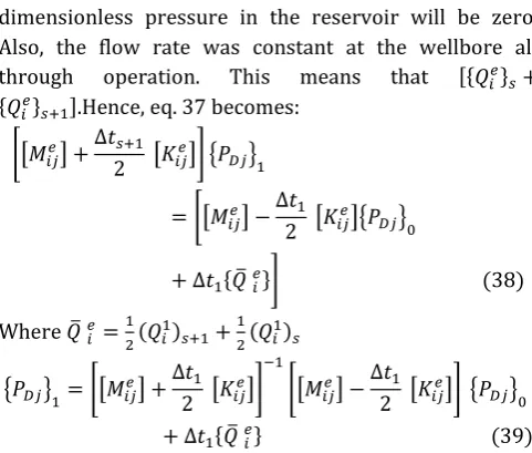
From the initial condition given in eq. 9 for a constant terminal rate case, it implies that when
s
0
, all dimensionless pressure in the reservoir will be zero. Also, the flow rate was constant at the wellbore all through operation. This means that [{ } { } ].Hence, eq. 37 becomes:[[ ]
[ ]] { }
[[ ]
[ ]{ }
{ ̅ }]
Where ̅
{ } [[ ]
[ ]]
[[ ] [ ]]{ }
{ ̅ }
7. RESULTS AND DISCUSSION
The steady state condition applies, after the transient period, to a well-draining a cell which has a completely open outer boundary. It is assumed that, for a constant rate of production, fluid withdrawal from the well will be
exactly balanced by fluid entry across the outer boundary and therefore,
onstant at i. e. , . , and
t and
This condition is appropriate when pressure is being maintained in the reservoir due to either natural water influx or artificially by the injection of some displacing fluid. The semi-steady state flow equations are frequently applied when the rate, and consequently the position of the no-flow boundary surrounding a well, is slowly varying functions of time. If the production rate of an individual well is changed, for instance, due to closure for repair or increasing the rate to obtain a more even fluid withdrawal pattern throughout the reservoir, there will be a brief period when transient flow conditions prevail followed by stabilized flow for the new distribution of individual well rates.
Thus, this solution of the diffusivity equation models radial flow of slightly compressible liquid in a homogeneous reservoir of uniform thickness; reservoir at uniform pressure before production; unchanging pressure at the outer boundary; and production at constant rate from a single well (centred in the reservoir) with wellbore radius.
The results obtained from this analysis were shown in the form of graphs of dimensionless pressure against dimensionless time. This was shown in Fig. 1. Fig. 1 is a log log plot of dimensionless pressure against dimensionless time. The graph shows for different dimensionless radii ranging between 1 and 1000000 in log cycles. It was seen from the graph that the dimensionless pressure history of the reservoir was not captured at the initial stage between the dimensionless time of zero and the respective dimensionless times in Fig. 1. This was due to the fact that, within these regions, the reservoir was at the infinite acting state. After these infinite acting period, it was observed that the dimensionless pressure increases and later becomes uniform became the withdrawn fluid has been completely replaced. This condition remains throughout the entire life of the reservoir presumably.
Fig. 1: Log-Log plot of PD against tD for various rD in the infinite acting regime
Table 1: Percentage error of FEM and Van Everdigen
4
,
5
.
1
n
r
eDr
eD
2
,
n
4
r
eD
2
.
5
,
n
4
r
eD
3
,
n
4
r
eD
3
.
5
,
n
4
r
eD
4
,
n
4
r
eD
6
,
n
4
D
t
% errort
D % errort
D % errort
D % errort
D % errort
D % errort
D % error0.05 0.4348 0.2 0.0000 0.3 0.0000 0.5 0.1621 0.5 0.4839 1 0.0000 4 0.2353 0.055 0.4167 0.22 0.0000 0.35 0.0000 0.55 0.1563 0.6 0.4511 1.2 0.1167 4.5 0.1515 0.06 0.0000 0.24 0.0000 0.4 0.0000 0.6 0.0000 0.7 0.4255 1.4 0.1105 5 0.1470 0.07 0.0000 0.26 0.0000 0.45 0.0000 0.7 0.0000 0.8 0.2699 1.6 0.0000 5.5 0.1431 0.08 0.0000 0.28 0.0000 0.5 0.0000 0.8 0.0000 0.9 0.3876 1.8 0.1014 6 0.1397 0.09 1.0274 0.3 0.0000 0.55 0.0000 0.9 0.0000 1 0.2488 2 0.0000 6.5 0.1368 0.1 0.0000 0.35 0.0000 0.6 0.0000 1 0.0000 1.2 0.2331 2.2 0.0951 7 0.1342 0.12 0.0000 0.4 0.0000 0.7 0.0000 1.2 0.0000 1.4 0.1106 2.4 0.0000 7.5 0.1319 0.14 0.0000 0.45 0.1748 0.8 0.1374 1.4 0.0000 1.6 0.1058 2.6 0.5425 8 0.1300 0.16 0.0000 0.5 0.0000 0.9 0.1325 1.6 0.1079 1.8 0.1019 2.8 0.0000 8.5 0.1281 0.18 0.0000 0.55 0.0000 1 0.0000 1.8 0.0000 2 0.0988 3 0.0000 9 0.1266 0.2 0.0000 0.6 0.0000 1.2 0.1227 2 0.0000 2.2 0.1921 3.4 0.0000 10 0.1238 0.22 0.0000 0.65 0.0000 1.4 0.0000 2.2 0.0000 2.4 0.0939 3.8 0.0000 12 0.1200 0.24 0.0000 0.7 0.0000 1.6 0.0000 2.4 0.0000 2.6 0.0920 4.5 0.0000 14 0.1174 0.26 0.0000 0.75 0.0000 1.8 0.0000 2.6 0.0000 2.8 0.0904 5 0.0000 16 0.0578 0.28 0.0000 0.8 0.0000 2 0.0000 2.8 0.0000 3 0.0000 5.5 0.0000 18 0.1144 0.3 0.0000 0.85 0.0000 2.2 0.0000 3 0.0000 3.5 0.0864 6 0.0755 20 0.1135 0.35 0.0000 0.9 0.0000 2.4 0.0000 3.5 0.0000 4 0.0845 7 0.0742 22 0.1129 0.4 0.0000 0.95 0.0000 2.6 0.0000 4 0.0000 5 0.0000 8 0.0000 24 0.1125 0.45 0.0000 1 0.0000 2.8 0.0000 4.5 0.0000 6 0.0000 9 0.0000 26 0.1123 0.5 0.0000 1.2 0.0000 3 0.0000 5 0.0000 7 0.0000 10 0.0000 28 0.0561
1E-10 1E-09 1E-08 0.0000001 0.000001 0.00001 0.0001 0.001 0.01 0.1 1 10
0.00001 0.0001 0.001 0.01 0.1 1 10 100 1000 10000 100000 1000000
L
o
g
Dim
ens
io
nles
s
P
re
ss
ure
Log Dimensionless Time
reD=1
reD=10
reD=20
reD=80
reD=100
reD=200
reD=500
reD=1000
reD=10000
reD=100000
Table 2: Dimensionless Pressure Distribution for
r
eD
1
.
5
,n
4
and
t
0
.
005
rD
tD 1 1.0625 1.1250 1.1875 1.2500 1.3125 1.3750 1.4375 1.5000
0.050 0.229 0.174 0.127 0.091 0.063 0.041 0.025 0.011 0.000
0.055 0.241 0.183 0.137 0.099 0.070 0.046 0.028 0.013 0.000
0.060 0.249 0.192 0.145 0.107 0.076 0.051 0.031 0.015 0.000
0.070 0.266 0.209 0.160 0.121 0.087 0.060 0.037 0.018 0.000
0.080 0.282 0.224 0.174 0.133 0.098 0.068 0.043 0.020 0.000
0.090 0.295 0.237 0.187 0.144 0.107 0.075 0.048 0.023 0.000
0.100 0.307 0.249 0.198 0.154 0.115 0.082 0.052 0.025 0.000
0.120 0.328 0.269 0.216 0.170 0.129 0.092 0.059 0.029 0.000
0.140 0.344 0.284 0.231 0.183 0.140 0.101 0.065 0.032 0.000
0.160 0.356 0.297 0.243 0.194 0.149 0.108 0.069 0.034 0.000
0.180 0.367 0.307 0.252 0.202 0.156 0.113 0.073 0.036 0.000
0.200 0.375 0.315 0.260 0.209 0.161 0.117 0.076 0.037 0.000
0.220 0.381 0.321 0.265 0.214 0.166 0.121 0.078 0.038 0.000
0.240 0.386 0.326 0.270 0.218 0.169 0.123 0.080 0.039 0.000
0.260 0.390 0.330 0.274 0.221 0.172 0.125 0.082 0.040 0.000
0.280 0.393 0.333 0.277 0.224 0.174 0.127 0.083 0.040 0.000
0.300 0.396 0.335 0.279 0.226 0.176 0.128 0.084 0.041 0.000
0.350 0.400 0.340 0.283 0.229 0.179 0.131 0.085 0.042 0.000
0.400 0.402 0.342 0.285 0.231 0.180 0.132 0.086 0.042 0.000
0.450 0.404 0.343 0.286 0.232 0.181 0.133 0.086 0.042 0.000
0.500 0.405 0.344 0.287 0.233 0.182 0.133 0.087 0.042 0.000
0.600 0.405 0.345 0.287 0.233 0.182 0.133 0.087 0.043 0.000
0.800 0.405 0.345 0.288 0.234 0.182 0.134 0.087 0.043 0.000
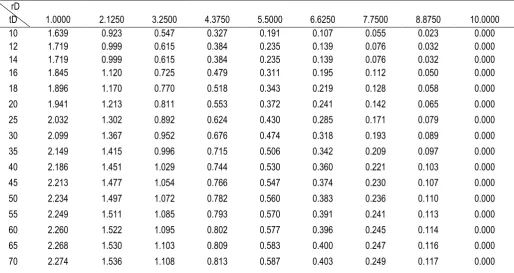
Table 3: Dimensionless Pressure Distribution for
r
eD
10
,n
4
and
t
0
.
05
rD
tD 1.0000 2.1250 3.2500 4.3750 5.5000 6.6250 7.7500 8.8750 10.0000
10 1.639 0.923 0.547 0.327 0.191 0.107 0.055 0.023 0.000
12 1.719 0.999 0.615 0.384 0.235 0.139 0.076 0.032 0.000
14 1.719 0.999 0.615 0.384 0.235 0.139 0.076 0.032 0.000
16 1.845 1.120 0.725 0.479 0.311 0.195 0.112 0.050 0.000
18 1.896 1.170 0.770 0.518 0.343 0.219 0.128 0.058 0.000
20 1.941 1.213 0.811 0.553 0.372 0.241 0.142 0.065 0.000
25 2.032 1.302 0.892 0.624 0.430 0.285 0.171 0.079 0.000
30 2.099 1.367 0.952 0.676 0.474 0.318 0.193 0.089 0.000
35 2.149 1.415 0.996 0.715 0.506 0.342 0.209 0.097 0.000
40 2.186 1.451 1.029 0.744 0.530 0.360 0.221 0.103 0.000
45 2.213 1.477 1.054 0.766 0.547 0.374 0.230 0.107 0.000
50 2.234 1.497 1.072 0.782 0.560 0.383 0.236 0.110 0.000
55 2.249 1.511 1.085 0.793 0.570 0.391 0.241 0.113 0.000
60 2.260 1.522 1.095 0.802 0.577 0.396 0.245 0.114 0.000
65 2.268 1.530 1.103 0.809 0.583 0.400 0.247 0.116 0.000
rD
tD 1.0000 2.1250 3.2500 4.3750 5.5000 6.6250 7.7500 8.8750 10.0000
80 2.282 1.544 1.115 0.819 0.592 0.407 0.252 0.118 0.000
90 2.286 1.548 1.119 0.823 0.594 0.409 0.253 0.119 0.000
100 2.289 1.550 1.121 0.825 0.596 0.410 0.254 0.119 0.000
110 2.290 1.552 1.122 0.826 0.597 0.411 0.254 0.119 0.000
120 2.291 1.552 1.123 0.826 0.597 0.411 0.255 0.119 0.000
130 2.291 1.553 1.123 0.827 0.598 0.412 0.255 0.119 0.000
140 2.291 1.553 1.123 0.827 0.598 0.412 0.255 0.119 0.000
160 2.292 1.553 1.124 0.827 0.598 0.412 0.255 0.119 0.000
The results presented in Fig. 1 are the dimensionless pressure at the wellbore at different dimensionless time for the case of constant pressure outer boundary condition. When a reservoir is opened for production, a pressure disturbance is created in the reservoir from the wellbore. This disturbance is not only felt at the wellbore but it travels through the entire reservoir formation to the external boundary. Therefore, Tables 2 and 3 shows the dimensionless pressure at different points within and outside the wellbore of the reservoir against their corresponding dimensionless time.
8. CONCLUSION
This paper has been able to present the pressure distribution across a bounded circular reservoir assumed to have constant terminal rate at the wellbore. The diffusivity equation was used to analyse the pressure in the system. It was shown from Figs. 1 that the dimensionless pressure increases drastically immediately this flow regime is attained. But as time increases, the dimensionless pressure variation flattens out asymptotically. The results obtained from this analysis showed that there was a strong correlation with the results obtained from the Van Everdigen and Hurst. It is important to note that the Van Everdigen and Hurst solutions only state the pressure at the wellbore at a particular time but this work predicts the pressure variation in the entire reservoir from the wellbore to the external boundary at the same time. These where shown in Tables 2 and 3 and it was noticed that the pressure decreases from the wellbore to the external boundary of the reservoir. Therefore the Finite element method has been used to approximate not only the values of the wellbore pressures for bounded circular reservoirs but also pressure outside the wellbore to the external reservoir boundaries.
9. REFERENCES
[1] Razminia K., Hashemi A., and Razminia A. A Least Squares Approach to Estimating the Average Reservoir Pressure. Iranian J. Oil & Gas Sci. Technol. 2(1), 22–32. 2013.
[2] Van Everdingen, A. F. and Hurst, W. The Application of the Laplace Transformation to Flow Problems in Reservoir. Trans., AIME 186, 305-324.1949.
[3] Essa K. S. M., Mina A. N., and Higazy M. Analytical Solution of Diffusion Equation in Two Dimensions Using Two Forms of Eddy Diffusivities. Rom. J. Phys. 56, 1228–1240. 2011.
[4] Oane M., Medianu R., Georgescu G., ToaderD., and Peled A. The determination of two photon thermal fields in laser-two-layer solids weak interactions using Green function method. Rom. Rep. Phys. 65, 997–1005. 2013.
[5] Timofte C. Homogenization Results for Hyperbolic-Parabolic Equations, Rom. Rep. Phys. 62, 229–238. 2010.
[6] Earlougher, R.C., Jr., Ramey, H.J., Jr., Miller, F.G., and Mueller, T. D. Pressure Distributions in Rectangular Reservoirs. J. Pet. Tech., 199-208. 1968.
[7] Momoniat E., McIntyre R. and Ravindran R. Numerical inversion of a Laplace transform solution of a diffusion equation with a mixed derivative term. Appl. Math. Comput. 209(2), 222–229. 2009.
[8] Miller, C.C., Dyes, A.B., and Hutchinson, C.A., Jr. The Estimation of Permeability and Reservoir Pressure from Bottom-Hole Pressure Build-Up Characteristics. Trans., AIME 189, 91-104. 1950. [9] Aziz, K. and Flock, D. L. Unsteady State Gas Flow –
Use of Drawdown Data in the Rediction of Gas Well Behaviour. J. Can. Pet. Tech., 2 (l), 9-15. 1963.
[11] Ramey, H.J., Jr. and Cobb, W. M. A General Pressure Build-up Theory for a Well in a Closed Drainage Area. J. Pet. Tech., 1493 -1505. 1971.
[12] Kumar, A. and Ramey, H. J., Jr. Well-Test Analysis for a Well in a Constant-Pressure Square. Soc. Pet. Eng. J., 107-116. 1974.
[13] Cobb, W.M. and Smith, J. T. An Investigation of Pressure Build-up Tests in Bounded Reservoirs," J. Pet. Tech. Vol 27, No. 8, 1975, pp. 991 – 997.
[14] Chen, H.K. and Brigham, W. E. Pressure Build-up for a Well with Storage and Skin in a Closed Square. J. Pet. Tech., 141-146. 1978.
[15] Chatas, A. T. A Practical Treatment of Non-steady-state Flow Problems in Reservoir Systems. J. Pet. Eng., B-44–56. 1953.
[16] John L. Well Testing, Soc. Pet. Eng. of AIME, New York. 1982.
[17] Mishra, S. and Ramey, H. J., Jr. A New Derivative Type-Curve for Pressure Build-up Analysis with Boundary Effects. Proc., 12th Workshop on Geothermal Reservoir Engineering at Stanford Univ., Stanford, CA, 45-47. 1987.
[18] Ambastha, K., Anil and Henry J. Ramey, Jr. Well-Test Analysis for a Well in a Finite, Circular Reservoir. Proc., 13th Workshop on Geothermal Reservoir
Engineering at Stanford Univ., Stanford, Califonia, 53-57. 1988.