* This paper is based on the author’s PhD dissertation at Staffordshire University. I thank Geoff Pugh, Bill Russe-ll, Nick Adnett, Peter Reynolds and Ahmad Seyf plus three anonymous reviewers for their many helpful suggestions. The remaining errors are the responsibility of the author.
** Received: June 4, 2010 Accepted: September 21, 2010
IDENTIFICATION ISSUES: A SURVEY
Bruno ĆORIĆ, PhD* Review article**
University of Split, Faculty of Economics, Split JEL: D53, G32, E22
bcoric@efst.hr UDC: 336.5
Abstract
If financial markets are perfect, the choice of the sources of finance does not influen-ce investment decisions. However, financial markets are considered to be far from per-fect. This review concentrates on the role of information asymmetry in determining real investment decisions. Despite the theoretical plausibility of a relationship between capital market imperfections and real investments, the empirical literature has found it difficult to identify this channel. Overall, more research is needed to identify a method that will not be subject to criticisms related to the use of cash-flow in the investment equation and will be based on the data that are relatively available across countries and over time.
Key words: investment, asymmetric information, capital markets imperfections
1 Introduction
of investment finance: equity finance, debt finance, or self finance. So, if financial markets are perfect, the choice of the sources of finance does not influence the firm’s investment decisions. However, the recent financial crisis has shown how far from perfect financial markets can be. This crisis has once again raised the issue of informational asymmetry in capital markets. It has demonstrated the possible consequences of capital market imper-fections for corporate investments and overall real economic activity. Although financi-al crises are not permanent but irregular events, the problem of asymmetric information is permanently present among participants in capital markets. Hence, capital market im-perfections can have a permanent influence on firms’ investment decisions and real eco-nomic activity. Analysis of corporate investment determinants has an important position in macroeconomics, industrial organization and corporate finance research. This review concentrates on developments and challenges in the empirical identification of the relati-onship between capital market imperfections and real investments.
The review is organized as follows. To motivate the discussion, section 2 considers groundbreaking studies which established the theoretical background of a channel linking information asymmetry in capital markets and investment decisions. Section 3 presents challenges in the empirical literature and methods used to identify this channel. Section 4 concludes.
2 Capital market imperfections: theoretical considerations1
2.1 Asymmetric information and equity finance
Information asymmetry in the equity market assumes that a firm’s management has more, or/and better, or/and “earlier” information about the true value of the firm’s existing assets, or/and the “quality” of its investment projects. An explanation of why firms can be unable or unwilling to raise funds in an equity market in the circumstances of asymmetric information is given by Greenwald, Stiglitz and Weiss (1984) and Myers and Majluf (1984). In these circumstances, a firm’s decision not to issue shares signals “good news” to investors while, conversely, this firm’s decision that it will issue shares signals “bad news” to investors. In particular, investors “read” the equity issue as a signal that the firm’s management, having “exclusive” information about the firm, considers existing share prices to be overvalued compared to the firm’s true value. Consequently, equity issue will induce a decrease in share prices and firm value. Since investors do not have full information about the firm’s true value, they “read” every equity issue in the same way. The consequence is that an equity issue decreases the firm’s share price, independently of the fact whether or not it is truly overvalued. This leads to misallocation of real capital, in the firm as well as at the aggregate level. Namely, even in cases when a project’s NPV
1 The problem of asymmetric information is not the only potential source of capital market imperfections. Other
is positive, firms will sometimes decide not to issue new shares and invest, because the decrease in share prices can outweigh any increase in value arising from the project’s positive NPV. Accordingly, in most cases firms will try to avoid equity issue as a source of financing new investment.
Since equity issue can lead to a decrease in a firm’s share price for reasons other than just asymmetric information, for example a change in the firm’s management in-centives (Greenwald, Stiglitz and Weiss, 1984), formal verification cannot rely on the test of whether share prices decrease when new shares are issued. It has to rely on proof that equity issue signals “bad news” for investors. Greenwald, Stiglitz and Weiss (1984) developed a model in which information asymmetry exists only in equity markets while in credit markets information is equally distributed between firms’ managers and outsi-de investors. In this two-period mooutsi-del each firm is characterised by net cash flow stre-aming from the firm’s existing operations, θ, and a set of new investment opportunities with return εQ(K) (where ε is a random variable, whose expected value is E(ε) = 1, vari-ance var(ε) =σε2, Q(K) denotes return on new investment and K is the level of investment.
The θ, which is different for different firms, symbolises the value of the firm’s existing assets, or the firm’s true “quality”. So, firms whose initial “qualities” (θ) are different have two possibilities to finance investments whose returns, Q(K), are assumed to be the same for all firms and investment opportunities. The first possibility is to use the equity market where investors do not observe the individual firm’s θ but only the average firm’s θ. The second possibility is the debt market where lenders observe θ. At the beginning of the period each firm determines the level of investment, K, issues equity in the amount e, or not, and finances the remaining investment amount by taking a loan in the amount b = K – e. Assuming the firms are risk-neutral, they act with the intention of maximizing firm value (T). More precisely, the firm (or the firm’s management) is supposed to act in a manner such as to maximise the value of the firm held by the “old stock holders”, which is represented by the following equation2,
(1)
Where V0 is the firm’s initial value, m stands for the weight that the firm places on its
initial as opposed to its terminal value. The term represents the share of the firm’s
assets that will be held by old stock holders at the end of the period. The term in square brackets stands for the firm’s value at the end of the period, which proceeds from the cash flows streaming from the existing firm’s operations, θ, and from the returns on the new investments, Q(K), minus debt obligations, b(1+R), where (1+R) represents the unit cost of the debt finance. Taken together, the second term on the right hand side of the equation (1) stands for the value of the old stock holders’ assets at the end of the period times the weight they place on that value as opposed to the initial value of their assets. Now, assuming that
2 To simplify presentation we excluded the cost of bankruptcy. This change does not influence any of the essential
every firm can choose between two sources of investment financing, if the firm chooses to use exclusively debt finance, its objective function (1), will be modified to:
TD = mV 0
D + (1 – m)θ + Q(KD) – KD (1 + R) (2)
If, on the other hand, it chooses full or partial equity finance then its objective function will be:
(3)
where e0 stands for the amount of equity the firm sells. V0D and V 0
E are initial values of
nonequity selling and equity selling firms, respectively. KD and KE are optimal levels of
investment for a nonequity selling and an equity selling firm, respectively. If we compare equations (2) and (3), we can gain insight into the possible difference in a firm’s value that is a consequence of different finance decisions. In the case of exclusive debt finance (2), the value of the old stock holders’ assets at the end of the period will be lower by the fixed amount of the debt repayment obligation, K(1+R). In the case of equity finance (3), the value of the old stock holders’ assets at the end of period, which proceeds from the same sources, will be lower by the proportion of the new owners’ share in the firm. That is, the
old stock holders will now receive only a fraction, , of the firm’s terminal value.
Since returns on new investment are assumed to be the same for all firms, it is possible, by using these modified objective functions, to simulate the firm’s finance decision rule and present it as a function, H, of the net cash flow, θ, streaming from the firm’s existing operations as follows,
(4)
or, in compressed form, as,
H (θ) = TD (θ) – TE (θ) (5)
Equations (4) or (5) have two implications. First, it is possible to calculate a certa-in theoretical level of θ, let’s say θ, where H (e θ) = 0, or in other words some level of cash e flows streaming from the existing firm’s operations for which TD (θ) = TE (θ), and the firm
is indifferent between debt and equity finance. Second, it also implies that
implies that the firm will use equity finance if its net cash flow is low, and debt finance where its net cash flow is high, or more precisely,
e = e0 if θ < θ; e = 0 if θ > e θ e (6)
The intuition is as follows. In both cases the old stock holders will give some amount of the cash flows streaming from the firm’s existing operations to finance new investment. In the case of debt finance that will always be a fixed absolute amount. In the case of equity finance that amount will be a fixed proportion of cash flows that are streaming from the firm’s existing operations. Hence, the burden of debt finance will be heavier to them in the case when the net cash flow, θ, is lower compared to the burden of equity finance, and vice versa.
Overall, this model formally demonstrates that firms with a low asset value will prefer to raise funds in the market, where potential outside investors are not able to observe their “quality”. Hence, firms entering the equity market will be adversely selected. Accordingly, any firm’s decision to issue shares will be read by incompletely informed outside investors as “bad news”, although that need not necessarily be the case.
2.2 Credit rationing
Credit rationing is broadly defined as a situation in which there exists an excess demand for loans because quoted loan rates are below the Walrasian market clearing level (Jaffe and Stiglitz, 1990:847). Theory of credit rationing aims to explain why the duration of such disequilibrium can be permanent, or at least too long to be explained by price persistence alone.
As in the case of the equity market, credit rationing theory rests on the assumption that a firm’s management and outside investors (intermediaries) do not share the same information about the firm and/or its projects’ qualities. In particular, the intermediaries (banks) who create supply in this market do not have full information about the “qualities” of firms’ projects. The consequences for the credit market can be demonstrated following the simple analysis by Waller and Lewarne (1994) of the demand and supply function in the credit market.
(7)
Where p is the probability that loans will be repaid, L is loan value and rL is the interest rate on loans. Taken together the first term represents the bank’s total revenue. The last two terms on the right hand side of the equation represent total costs. Where D stands for the total value of deposits, rD is the interest rate on deposits, and q stands for the cost parameter of servicing loans.
The relation between the amount of loans supplied and deposits the bank collects can be defined as D = bL, where b is the deposits to loans ratio, and where b ≥ 1, meaning that, due to reserve requirements, the amount of loans the bank supplies is equal to or lower than the amount of deposits it has collected. In that case the bank’s profit maximization function can be rewritten as follows,
(8)
Maximising equation (8) with respect to L yields the loan supply curve (LS).
(9)
From equation (9) it is not difficult to calculate that loan supply is a continuously
increasing function of the loan interest rate , since p>0 and q>0. Hence, the
deduced loan supply curve can be presented (by inverting this derivative) as a standard supply curve.
This implies that any excess demand for loans will be eliminated by increasing the loan interest rate, as in any “standard” market. Therefore, any permanent disequilibrium is not possible in this market. The only thing that can happen is short-term excess demand, which will last only as long as the loan interest rate does not rise enough to restore a new, market-clearing equilibrium. Even if, for some reasons, the probability of repayment (p) decreases, the loan supply curve, although steeper, will still be an increasing function of the loan interest rate. The equilibrium amount of loans will then be smaller but the above conclusions and their implications will be unchanged. Hence, the feature that loans may not be repaid due to default is not enough to produce credit rationing, that is, permanent disequilibrium in the loans market. However, if we include the assumption that the probability of loan repayment (p) is dependent upon the loan interest rate (or, more precisely, that the probability of loan repayment is inversely related to the interest rate)
(10)
(11)
It is not difficult to calculate that the slope of this new loan supply curve is not the same as before and that now the slope is,
(12)
where is the elasticity of the probability of loan repayment with respect to the
interest rate. The ep measures the percentage change in the probability of loan repayment
in response to one percentage change in the loan interest rate, and is negative by assump-tion from equaassump-tion (10), . The ep makes it possible to demonstrate that the loan
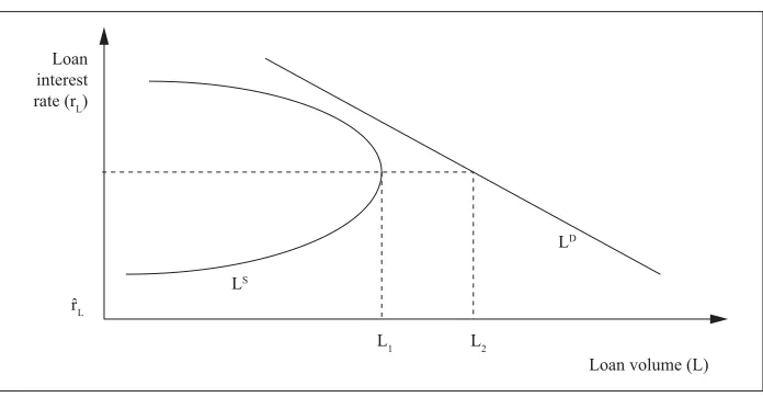
supply function is not always a continuously rising function of the interest rate, but that at some point it can become a decreasing function of the interest rate. This key element of credit rationing theory can be graphically presented by figure 1.
Figure 1: Market for loans with a backward bending supply curve
Loan interest rate (rL)
rˆL
Loan volume (L) L1
LS
LD
L2
This implies that the quantity of loans supplied increases with the interest rate only until the loan interest rate reaches the turning point, reL. If at that interest rate excess demand for loans is still present in the market, then the market will be characterised by permanent disequilibrium. The excess demand for loans in that case will not be eliminated by a rising loan interest rate, as standard economic theory assumes, for above reL a bank’s profit decreases with the loan interest rate and it will be willing to offer not more but fewer loans at higher interest rates. The intuition behind this is as follows. Increases in the interest rate have two effects on bank profit. The first is positive and leads to an increase in a bank’s profit, because every loan now is charged at a higher interest rate. The second effect is negative and leads to a decrease in a bank’s profit, because a rise in the interest rate brings about a decrease in the probability that loans will be repaid (equation 10). When the loan interest rate is above reL, the second effect outweighs the first, meaning that the increase in the interest rate will reduce the bank’s profit, hence loan supply will decrease. Consequently, the market loan interest rate will stay persistently at the reL level despite the existence of excess demand for loans at that level of rL.
2.3 Adverse selection and incentive effects
The possibility of credit rationing relies on the assumption that loan repayment probability is inversely related to the interest rate. Stiglitz and Weiss (1981) provided two basic explanations for this assumption: adverse selection and incentive effects.
The adverse selection effect assumes that asymmetry in information arises ex-ante. It suggests that the mix of applicants changes adversely as the interest rate increases. In other words, as the interest rate rises borrowers from whose projects banks have higher expected revenues (safer projects) drop out of the market and the market becomes do-minated by borrowers from whose projects banks have lower expected revenues (riskier projects). Since banks cannot distinguish among different type of borrowers, they charge them all the same interest rate. So, the change in the mix of applicants will shrink total bank revenue and hence profit. The main reason behind this adverse selection effect is that in the case when an investment project is financed by debt (fixed repayment obligation) any increase in project riskiness changes banks’ and firms’ expected profit in the opposi-te direction. From the firms’ point of view, expecopposi-ted profit increases with riskier projects. Conversely, from the bank’s point of view expected profit decreases with project riskine-ss. As the interest rate rises, firms’ cost of project financing increases, so firms with less profitable, hence less risky, projects, drop out of the market one by one. The consequen-ce is a change in the mix of loan applicants that banks faconsequen-ce. The average project is now more risky, hence less profitable for the bank.
Stiglitz and Weiss (1981) constructed a model in which economic agents who want to invest have to borrow money from banks3. Each firm (borrower) is endowed with the
same size project, L, and all those projects have the same expected mean return E(R). The only difference among firms is in the projects’ riskiness. Different projects have different probability distributions of project returns, f(R,θ); where θ represents the dispersion of a
3 To simplify presentation we excluded collateral. This change does not influence any of the essential features
project’s returns around its expected value, E(R), and where higher θ corresponds to a gre-ater risk in the Rothschild and Stiglitz’s (1970) “mean preserving sense”.4 For example,
figure 2 presents two projects. As we can see projects 1 and 2 have the same mean expec-ted returns, but the returns probability distribution function, f(R,θ2), has more weight on its tails. Hence, project 2 is riskier in the Rothschild and Stiglitz (1970) “mean preserving sense” than project 1. Stiglitz and Weiss (1981) also assume that banks are not able to observe individual firms’ project riskiness, θ. Hence, they charge all loan applicants the same loan interest rate, r. Accordingly, the revenue banks will earn from the loan depen-ds on both the interest rate they charge and the return realization of the financed project. The bank’s revenue function can be represented as follows,
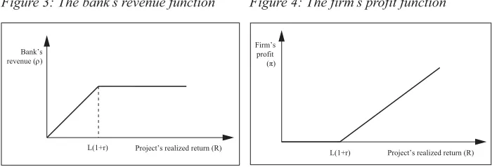
ρ(R, r) = min(L (1 + r); R) (13)
where ρ denotes the bank’s revenue. R is the project’s realized return. r stands for the loan interest rate. Finally, L is project size and also loan size. Equation (13) implies that the bank will receive full loan repayment L (1+r) if the project’s realized return is R > L (1+r). Conversely, if R is lower than the loan repayment then the firm will declare bankruptcy and the bank will receive only R. Figure 3 below depicts the bank’s revenue (13) condi-tioned upon the project’s realized return. As we can see, the bank’s revenue function is a concave function of the realized project returns, for the bank’s revenue from the project increases up to the point at which the realized project returns reach the amount necessary for full loan repayment. After that point, the bank’s revenue stays constant, because it is independent of how much the realized project returns increase.
The firm’s earnings from the project also depend on the interest rate the bank charges and the return realization of its project. However, the limited liability assumption makes the firm’s profit function as follows,
π(R, r) = max(R – L (1 + r); 0) (14) This means that the firm’s profit from the project will be R – L (1 + r) in cases in which project return realization is R > L (1 + r). Conversely, if R < L (1 + r) then the firm will declare bankruptcy and its profit will be 0. Figure 4 below depicts the firm’s profit function (14) conditioned upon the project’s realized return. As we can see, the firm profit function is a convex function of realized project returns. In other words, the firm’s profits (losses) stay at zero up to the point where realized project returns fall short of the amount neces-sary for full loan repayment. Above that point, the firm’s profit increases proportionally
4 Rothschild and Stiglitz (1970) addressed the question of in which case a random variable Y is more variable
(more risky) than another random variable X with the same expected value. There are at least four plausible answers to this question. These are: Y is equal to X plus noise; all risk averters prefer X to Y; Y has more weight in the tails than X; Y has a greater variance than X. Rothschild and Stiglitz (1970) demonstrated that the concept of increasing risk is not equivalent to that implied by equating risk of X with the variance of X. They showed, that is, that the first three approaches lead to a single definition of greater riskiness, different from that of the fourth approach. Using Stiglitz and Weiss’s (1981) notation from above Rothschild and Stiglitz’s (1970) definition of greater riskiness can be formu-lated as follows. Between two projects that have the same mean expected return, ∞
0Rf (R, θ1)dR =
∞
0Rf (R, θ2)dR, risk-averse economic agents will prefer the project with dispersion θ1 to the one with θ2 if, a
0F (R, θ1)dR =
a
with realized project returns. If we consider the firm’s profit function (figure 4) and pro-ject returns probability distributions (figure 2) together it is possible to provide an intuiti-ve explanation of why in a case in which projects are financed by debt, the firm’s expec-ted profit increases with the project risk. As we can see, a riskier project, with dispersi-on θ2, is more profitable to the firm simply because the probability of favourable events, high return realizations and high profits associated with those returns, is greater than for a project with dispersion θ1. Symmetrically, the probability of unfavourable events, low return realizations and the associated bankruptcy is greater for the project with θ2 than for the one with θ1. However, the losses the firm will suffer in those circumstances are limited to zero by the firm’s limited liability assumption. Under assumption that cost of financing, r, is the same for both projects this implies that from the firm’s point of view the expectedprofitability of the riskier project 2 is higher than the expected profitability of the less risky project 1. Therefore, as the cost of project financing, r, increases, firms with less profitable (projects with lower expected profitability) and at the same time less risky projects, drop out of the market one by one. The consequence is a change in the mix of loan applicants that banks face.
Probability distributions of project returns
Project returns R E(R)
0
f (R, θ2)
f (R, θ)
f (R, θ1)
Bank’s revenue (r)
Project’s realized return (R) L(1+r)
Figure 2: Project returns probability distributions
Figure 3: The bank’s revenue function
Firm’s profit (π)
Project’s realized return (R) L(1+r)
In a more formal way, it is possible to formulate the firm’s expected profit function (Π) as a function of the interest rate banks charge (r) and the dispersion of project returns around its mean expected value, that is, project riskiness (θ)5
Π (r, θ) = ∫∞0 max [R – L(r + 1); 0]dF (R, θ) (15)
where the firm’s expected profit is an increasing function of project riskiness, ,
for the reasons explained above, and a decreasing function of interest rate, ,
sim-ply because an increase in interest rate raises the cost of project financing. From equation (15) it is possible to find, for a given interest rate, some threshold level of project riskiness ( θ) for which the expected profit level is equal to zeroe
Π (r, θ) = e ∫0∞ max [R – L(r + 1); 0]dF (R, θ) = 0e (16)
At that interest rate only firms whose project riskiness is higher than the threshold value, θ, (θ > e θ) will apply for loans and undertake projects, simply because only those e firm’s projects will be profitable. All other firms, whose project riskiness is, θ < θ will e find it unprofitable to undertake projects and will drop out of the loans market. The rela-tion between the interest rate, r, and the threshold project riskiness value, θ, can be obta-e ined from the total differential of the above firm’s expected profit function (16)
(17)
from which we can express the derivative of the threshold project riskiness level, θ, upon e loan interest rate, r, as:
(18)
Equation (18) indicates a positive relation between the interest rate and the threshold project riskiness level. More precisely, it indicates that an increase in the interest rate leads to an increase of the threshold project riskiness level ( θ), that is the level of project riski-e ness below which the firm does not apply for loans and does not undertake investment projects. Therefore, as the loan interest rate increases, the threshold level of project riski-ness, θ, rises and firms with less risky projects one by one leave the credit market, there-e by changing the mix of projects in the market in favour of higher risk projects.
5 The difference between the firm’s profit (14) and the firm’s expected profit function (15) is that the latter is no
If we now consider the bank revenue function (figure 3) and project returns probabi-lity distributions (figure 2) together, it should become clearer why this change in the mix of applicants is unfavourable to the bank. As we can see, the riskier project, with dispersi-on θ2, is less profitable to the bank simply because the probability of unfavourable events, low return realizations and low revenues (losses) associated with those returns is greater than for the project with dispersion θ1. Again, the probability of favourable events, high return realizations and associated high revenues is greater for project θ2 than for θ1. Yet the revenues the bank receives in this case are limited by the size of the loan repayment rate, L(1+r). From the bank’s point of view this implies that expectedprofitability from the ri-skier project 2 is lower than expected profitability from the less risky project 1. Consequ-ently, a change in the mix of loan applicants from low to higher risk, caused by an incre-ase in the loan interest rate, hurts bank profitability. Hence, the bank’s profit will not be a continuously increasing function of the loan interest rate, but will, actually, start to dec-line, with the bank’s loan supply, above some interest rate level, say r, as we have shown i in the previous section.
Contrary to the adverse selection effect, the adverse incentive effect or moral hazard problem takes place once the loan has been received. The adverse incentive effect assu-mes that asymmetry in information arises ex-post because banks cannot observe which type of project the firm actually undertakes. For the reasons explained above, higher in-terest rates will induce borrowers to undertake riskier projects. The change in the mix of undertaken projects will shrink banks’ expected revenue (profit) and will cause a fall in the loan supply above some level of the interest rate.
The outcome of these findings is straightforward. Insofar as firms very often are not willing to enter the equity market due to the asymmetric information problem, the exi-stence of credit rationing in the loans market implies that firms’ ability to raise investment funds externally can be constrained. Hence, a firm’s investment will not be determined just by the NPV of its projects but also by the availability of an internal source of finance.
will be asked to pay on external funds. Hence, the firm’s investment level will again be affected by the availability of internal source of finance.
This review illustrates only the basic theoretical background of the channel linking capital market imperfections and asymmetric information in the equity and credit markets. The above considered groundbreaking studies have inspired an enormous literature about the sources, kinds and consequences of information asymmetry in capital markets (seminal contributions include: Bester, 1985; Gale and Hellwig, 1985; De Meza and Webb, 1987, 1992; Williamson, 1987; Diamond, 1991; Boot and Thakor, 1993; Pagano and Jappelli, 1993; Holmstrom and Tirole, 1997; more recent ones include: Hellmann and Stiglitz, 2000; Clementi and Hopenhayn, 2006; Inderst and Meller, 2007; Arnold and Riley, 2009; Morellec and Schurhoff, 2010; Tinn, 2010).
3 Identification issues
Despite the theoretical plausibility of a relationship between capital market imperfections and investment, empirical literature has found it difficult to identify this channel. The main problem of this literature is the inability directly to observe and measure the external finance premium. Faced with that obstacle, researchers have developed various estimation strategies. The literature was initiated by Fazzari, Hubbard and Petersen (1988) (FHP). FHP used a Tobin Q investment model to test for the effect of capital market imperfections on firms’ investment. Tobin’s Q theory of investment formalizes the Keynesian notion that the incentive to built new capital depends on the market value of the capital relative to the cost of constructing this capital. If an additional unit of installed capital raised the market value of the firm by more than the cost of acquiring the capital and putting it in place, then a value-maximising firm should acquire it and put it in place. To capture this notion in an observable quantitative measure, Tobin defined the variable q to be the ratio of the market value of a firm to the replacement cost of its capital stock. He then argued that investment is an increasing function of q. The Q theory of investment is based on the notion that all relevant information is captured by the market valuation of the firm, and therefore other variables such as cash flow, profit, or capacity utilization should have no additional predictive power for investment (Abel, 1990). FHP estimated the following Tobin’s Q investment model for a panel of manufacturing firms
(19)
case in which this is true, the estimated coefficient on variable which measures firms’ internal sources of finance should be positive and statistically significant when it enters the investment regression equation. Moreover, its inclusion should increase the explanatory power of the standard investment specification. On the other hand, if financial markets are frictionless, as in the Modigliani and Miller (1958) model, then the estimated coefficients on the internal sources of finance variable should not be statistically different from zero. In additional, it should not increase the explanatory power of the investment equation model. The problem with this conclusion is the well-known objection that cash flow gains significance in investment equations only because of its predictive power over the expected investment profitability. To avoid these objections FHP divided firms into different categories, according to the likelihood of facing financial constraints when they raise investment funds externally, and estimated equation (19) for each group of firms separately. The criterion used for this purpose was the firms’ profit retention ratio, that is, their dividend policy. Namely, according to FHP if the external costs of finance are higher than the internal resources, then it is not optimal for the firm to pay dividends and finance profitable investment opportunities from external sources. So, the firms which had the lowest dividends to income ratio in the sample were classified into the class of firms that are most likely to face financial constraints (Class 1). On the other hand, the class of firms for which the probability of facing financial constraints was the lowest were those with the highest dividends to income ratio in the sample (Class 3). Finally, the firms whose retention ratio was between these categories were allocated to Class 2. The results were in line with the prediction of the capital market imperfection theory. In particular, the cash flow coefficient in the equations they estimated had a uniformly positive sign and declined monotonically through firm classes. It was almost three times larger for Class 1 firms than for Class 3 firms, with Class 2 firms positioned between those two estimates. As a result of the inclusion of cash flow into the standard Tobin Q model of investment, the explained proportions of the variance of I/K increased for all firm classes. Moreover, adding the cash flow increased the adjusted R2 most for Class 1 and least for Class 3.
Some authors raised concerns that dividend payment is an imperfect sample split criterion. Without an explicit modelling of why firms pay dividends we can not be sure that firms which do not pay dividends are financially constrained and vice versa. For example, if the cutting of dividends is taken to be a negative signal, many financially constrained firms may be “forced” to proceed with the same dividends payment strategy despite the problems they face (Devereux and Schiantarelli, 1990). A decrease in the firm’s value which would arise due to missing a positive investment opportunity can be lower than a decrease which would arise due to a decrease in share prices. Concerned with this possibility, some authors have used different kinds of sample division.
empirical analysis revealed that the Japanese firms which are not affiliated with this industry group are much more sensitive to fluctuations in internal sources of finance than keiretsu members. The same results were obtained by Schaller (1993) who separated his sample of Canadian firms based on their membership of an industry group. Devereux and Schiantatareli (1990), Gertler and Gilchrist (1994), Gilchrist and Himmelberg (1995) and Vermeulen (2002), have argued that firm size is the proper sample criterion. Since larger firms are usually more mature businesses with long established reputations, they are less likely to suffer from asymmetric information problems. The same reasoning induced Schaller (1993) to classify firms according to their age. The possession of a bond rating was proposed by Whited (1992) and Gilchrist and Himmelberg (1995) as another sample division criterion. The intuition behind it was the signalling effect of bond rating. The same intuition led Calomiris, Himmelberg and Wachtel (1995) to divide their sample into two groups comprising those companies that issue commercial papers and those that do not. In general, the studies, irrespective of specific sample split criteria, find a much stronger effect of changes in internal funds on investment for the groups of firms which they classified as financially constrained.
However, all the above sample split criteria can be criticized as incomplete (Hu and Schiantarelli, 1998). First, the probability that some firm faces financial constraints is a function of many factors. Hence, the reliable sample split criterion must include and pro-perly evaluate all these factors. Second, the firm’s position on this “scale” is not fixed and independent of its activities. In other words, a firm can become more or less constrained over time. Therefore, any classification into groups that are fixed through a sample peri-od is not appropriate. As a remedy Hu and Schiantarelli (1998) proposed the endogeno-us switching regression model in which each firm in each time period can operate in eit-her a financially constrained or unconstrained regime. The probability for any firm to be classified in one of these regimes is determined by the switching function, which inclu-des both firms’ financial variables (debt to asset ratios, interest expense to income ratios, liquid financial asset to capital ratios) and non financial variables (size, bond rating). The regression analysis they conducted, using this sample split technique, confirmed earlier FHP findings. The same sample split criterion, with the same outcome, was also used by Hovakimian and Titman (2006), and Almeida and Campello (2007).
lite-rature, for example: the sales accelerator approach (FHP, Vermeulen, 2002); Jorgenson’s neoclassical formulation (FHP); the error correction model (Bond, Elston, Mairesse and Mulkay, 2003); Euler equation of the dynamic optimization problem of firms (Whited, 1992; Bond and Meghir, 1994; Hubbard, Kashyap and Whited, 1995; Bond, Elston, Mai-resse and Mulkay, 2003); and different combinations of those approaches (Hoshi, Kashyap and Scharfstein, 1990, 1991; Audretsch and Elston, 2002). Yet, among all these specifica-tions only Tobin’s Q investment theory explicitly claims to be able to control for changes in investment opportunities. Proponents of the Tobin Q investment specification argue that average q on the right hand side of Equation (19) is a good proxy for this information. If average q effectively controls for the effects of changes in investment opportunities, the significance of cash flow should contain information only on financial constraints. Anot-her problem is that cash flow is only one part of firms’ internal source of finance. Partly due to this reason, and partly because of the previously mentioned problems with cash flows, some authors (Hoshi, Kashyap and Scharfstein, 1991; Vermeulen, 2002) construc-ted and used other proxies for the internal source of finance. Some of these are: the amo-unt of short-term securities at the beginning of the period; total debt as a fraction of total assets and short-term debt as fraction of short-term assets. In general, the results obtai-ned by these measures of internal sources of finance confirmed the previously mentioobtai-ned findings, despite the results being less strong and significant. The problem with most of these measures is that they measure the book rather than the market value of a firm’s in-ternal sources of finance. Hence, there is no guarantee that they are able to correctly pick up the effects of economic shocks on firms’ internal sources of finance. Overall, although cash flow is an imperfect proxy for internal sources of finance, its widespread use arises due to the fact that it is the only such measure available for internal sources of finance in most cases (Hubbard, 1998).
The most serious criticisms of the FHP methodology come from the recent resear-ches of Kaplan and Zingales (1997), Gomes (2001), Alti (2003), Cummins, Hassett and Oliner (2006), and Whited (2006).
The Kaplan and Zingales (1997) (KZ) objection to the FHP approach is two-fold. First, they disqualified FHP’s empirical findings and claim to have obtained opposing results when examining the FHP data sets in more detail. Second, they argue that there are no prior theoretical reasons to assume that investment cash flow sensitivity is monotonically increasing in the degree of financing constraint.
constraints on investments. Following KZ, Cleary (1999) obtained the same results for a larger sample (1,317 firms) of the US firms.
FHP (2000) challenged these results on several grounds. First, since firms are not obli-ged to declare explicitly whether or not they face difficulties in financing their investment, this criterion is ambiguous. Second, firms’ cash stocks, unused credit lines and levera-ge are also not an appropriate measure of financial constraints. Firms can have high cash stocks or keep unused credit lines not because they do not face constraints in attempts to raise external funds, but quite the opposite. A forward looking firm aware that it may face problems of raising external finance, may find it reasonable to keep large cash stocks and unused credit lines as precautionary buffer stocks. Finally, a low leverage level also does not necessarily mean that the firm is not credit constrained but can also signal that the firm is not able to obtain credit. Overall, according to FHP (2000) KZ’s empirical results come from the fact that their methodology tends to classify financially distressed firms as constrained. Since financially distressed firms are more likely to use cash flow to enhan-ce liquidity, repay loans and avoid bankruptcy than to finanenhan-ce investment, the KZ findin-gs should not be surprising. They are a product of a wrong classification strategy rather then a proof that the FHP methodology is incorrect (FHP, 2000).
The second KZ objection to the FHP methodology is theoretical. KZ argue that there are no strong theoretical reasons to expect that investment-cash flow sensitivity increases monotonically with the degree of financial constraints. In other words, the effect of changes in firms’ internal source of finance (measured by cash flow) on investment is not necessarily the strongest for the financially most constrained firms and vice versa. According to KZ a firm is supposed to choose the optimal level of investment in fixed capital (I) to maximize the following objective function
max[F(I) – I – C(E, k)]; I = W + E (20)
where F(I) is a single factor production function with standard properties (F’ > 0, and F’’ < 0). The sources of investment finance are external (E) and internal funds (W). Due to asymmetric information, agency costs or risk aversion, external funds generate additional costs, which are represented by the cost function C(E,k), where E is the amount of external funds used to finance investment and k is the measure of firms’ wedge between the cost of funds raised internally and externally. Furthermore, C is assumed to be convex in E. So, the first term in the square brackets represents revenues from investment and the last two terms stand for costs of investment. Taking internal funds (W) and the wedge between costs of internal and external funds (k) as given, the firm’s task is to choose the level of investment (I) which maximises their profit. The first-order condition for profit maximization of (20) is,
F1(I) – 1 – C1 (I – W, k) = 0 (21)
(22)
where F11 represents the second derivative of F with respect to I. C11 is the second partial
derivative of C with respect to its first argument, is clearly positive as far as C11 is
greater than zero and F11 is negative as assumed above. That is, the firm’s investment (I) increases with the availability of internal funds (W) if the firm is financially constrained. On the other hand, if capital markets are frictionless, then the internal source of finance does not affect investment decisions (dI/dW = 0, since C = 0 and then C11 is also 0). Hence, it is clear that changes in internal funds influence the investment of financially constrai-ned firms. Yet, something that is not clear, according to KZ, is the statement that the in-vestment cash flow sensitivity (dI/dW) should monotonically decrease with respect to W. In other words, there is no reason to expect that the same change in internal funds (ΔW) would induce a smaller change in the investments of a firm with high internal funds, than in the investments of a firm with low internal funds. This can be seen if we calculate the change in investment-cash flow sensitivity with respect to W from equation (22)
(23)
Transforming (23) we can express it as
(24)
where F111 represents the third derivative of F with respect to I. C111 is the third partial de-rivative of C with respect to its first argument. Given that the second term is always po-sitive, change in investment-cash flow sensitivity with respect to W, d2I/dW2 is negative
only if the first term (F111/F2
11 – C111/C
2
11) is negative. To be fulfilled, this condition asks
for a certain relationship between the form (curvature) of the production function (F) and the external funds cost function (C1). Hence, change in investment-cash flow sensitivi-ty with respect to W (d2I/dW2) is not universally negative. This can be presented
graphi-cally as in FHP (2000).
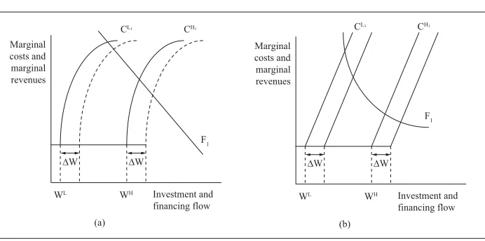
Figure 5 presents the investment market graphically. The quantity of capital the firm invests and the price of that capital is determined by the intersection of demand (F1) and supply of capital (C1). The firm’s capital (investment) demand function, F1, is a decrea-sing function of the cost of funds. The capital supply function is horizontal up to the point beyond which the firm’s investment cannot be financed by its own funds, where WL
de-notes low and WH a high quantity of internal funds. The horizontal segment indicates the
constant marginal cost of investment funds the firm faces for internal finance. After that point, the capital supply function is increasing (C11>0). The positive slope segment indi-cates the rising marginal costs the firm faces when it raises external finance above its in-ternal sources. So, CL
1 and C H
and high internal funds respectively. As we can see, the effects of a change in internal funds (ΔW) on the firm’s investment depend on the firm’s initial level of internal funds and on the shape of the capital demand and supply functions. So, the same change in internal funds (ΔW) would induce a larger change in the investments of a firm with high internal funds (WH) than in the investments of a firm with low internal funds (WL) (in other words,
investment-cash flow sensitivity (d2I/dW2) would be positive) when, for example6:
• the capital supply function (C1) is concave (C11>0, C111<0) in their external finan-ce part and the capital demand function (F1) is linear (F11<0, F111=0) as in figure 5, panel a7;
• or when the capital supply function (C1) is linear (C11>0, C111=0) and the capital de-mand function (F1) is convex (F11<0, F111>0), as in figure 5, panel b.8
According to FHP (2000), the KZ model misses the point and does not provide a tique of this literature. They argue that the level of the firm’s internal funds, W, is not a cri-terion that classifies firms as financially constrained or unconstrained. None of the studies in this literature uses the level of the firm’s internal funds, W, as a sample division crite-rion. Firms should be classified based on intrinsic characteristics that make them more or less exposed to the asymmetric information problem. The firms that are more exposed to asymmetric information will face higher costs per unit of external finance. Hence, their changes in investment due to changes in internal sources (dI/dW) should be larger. The
6 It is possible to figure out other cases when (d2I/dW2) would be positive. However, for the validity of KZ argu-mentation it is sufficient that there exists at least one such case. Hence, due to space limitation we illustrate only cases which are originally considered by KZ.
7 The capital supply function (C
1) can be concave, if for example the firm exhibits economy of scale when
rais-ing external funds. Namely, if the firm raises external finance by bond issue, then marginal costs decrease with the size of the bond issue, due to fixed costs accompanying the issuance.
8The capital demand function (F
1) can be convex if, for example, the firm production function exhibits decreas-ing returns on capital investment.
Figure 5: KZ Investment demand and investment funds supply functions
F1
WL
Marginal costs and marginal revenues
Investment and financing flow
∆W ∆W
WH
(a)
CL1 CH1
F1
WL
Marginal costs and marginal revenues
Investment and financing flow
∆W ∆W
WH
(b)
necessary condition for dI/dW of financially constrained firms to be larger than dI/dW of financially unconstrained firms according to (22) is,
(25)
from which, by rearranging, we obtain,
(26)
According to FHP (2000), there are no prior reasons why the firm production functi-on (F) should be systematically different between cfuncti-onstrained and uncfuncti-onstrained firms. Hence, the only necessary condition that should be fulfilled for the investment of finan-cially constrained firms to be more sensitive to changes in W compared to finanfinan-cially un-constrained firms’ investment is C
11
Constrained> C 11
Unconstrained. That is, constrained firms
sho-uld face a relatively steep capital supply curve, above their internal funds level, com-pared to unconstrained firms. A graphic presentation of this argument should make this more appealing.
Figure 6: FHP investment demand and investment funds supply functions*
F1
CL1
Marginal costs and revenues
Investment and financing flow ∆W
CH1
*The diagram assumes that capital supply curve is linear (C11>0, C111=0). The conclusion does not change if we assume that capital supply curve is concave (C11<0, C111<0) as in figure 5 panel (a).
Gomes (2001) and Alti (2003) reconsidered the well known question about the abili-ty of average q to measure future investment opportunities, as well as a possible spurious correlation between investment and cash flow.
Gomes (2001) developed a formal model of investment and created two sets of artifi-cial firm-level data. In the first variant of the model finanartifi-cial market frictions were expre-ssed by transactions costs arising from the firm’s external financing. In the second variant of the model these transaction costs were equalized to zero. Firms in both models were supposed to maximize their profits over time by making a decision about participation in the goods’ market, the level of investment and the source of finance. Tobin’s Q inves-tment equation augmented by a cash flow variable was estimated for each data set sepa-rately. The estimated coefficient on cash flow obtained from the first data set appears to be significant. However, the cash flow was also significant in the equation estimated by the second data set. More importantly, the addition of the cash flow variable to the Q in-vestment formulation does not add any new explanatory power to either regression. Con-sequently, according to Gomes (2001), not only is the existence of financial constraints insufficient to establish cash flow as a significant regressor beyond average q, but it also appears not to be necessary. The correlation between investment and cash flow arose due to the strong colinearity between average q and cash flow in his model. Hence, it is possi-ble that measurement error in the construction of average q reduces correlation between average q and investments. Consequently, it generates a spurious correlation between cash flow and investment, and induces the increase of adjusted R2 when cash flow is added to
the investment equation. In other words, it is possible that all the investment equations’ characteristics, observed by many authors in real data, are the result of imprecise measu-rement of average q. To illustrate this point, Gomes (2001) introduced measumeasu-rement errors of average q in the artificial data set and estimated investment regression for this data set. The regression results revealed that inclusion of cash flow in Tobin’s Q investment equa-tion in this case does increase the explanatory power of the investment equaequa-tion.
In a separate line of research, Erickson and Whited (2000), Cummins, Hassett and Oliner (2006), and Whited (2006) found that the cash-flow effect in investment regressi-ons greatly diminishes when measurement errors in average q are taken into account. No-tably et al. (2006) employ the firm-specific earnings forecasts from securities analysts to construct a measure of average q. Average q is supposed to measure the ratio of the firm’s intrinsic value to the replacement costs of its assets. Since the firm’s intrinsic value is uno-bservable, its market value is usually employed as a proxy of its intrinsic value. However, the stock market may measure the firm’s intrinsic value with considerable and persistent error. To investigate this potential source of measurement error, they used the firm-specific earnings forecasts from securities analysts to construct a measure of average q that need not rely on the stock market. The results of their analysis revealed that after controlling for fundamentals using the analysts-based average q, investments appear to be insensiti-ve to cash flow, einsensiti-ven for firms typically thought to be liquidity constrained.
These recent researches have produced three results that cast doubt on the eviden-ce for financing constraints from the studies based on FHP methodology. First, assuming that financing constraints exist, the size of the estimated cash-flow coefficient need not be positively related to the degree of the constraints. Second, positive cash-flow coeffici-ents can be generated without any financing constraints. Finally, the cash-flow effect eit-her disappears or becomes much smaller when one controls for the measurement error in q (Cummins, Hassett and Oliner, 2006). Taking these objections into account, some aut-hors proposed estimation methods that should overcome these identification problems.
Hovakimian and Titman (2006) tested the sensitivity of firms’ investment to cash funds raised from voluntary asset sales. The cash obtained from voluntary sales of assets, which are not related to the firm’s main business, is less likely to be correlated with the sellers’ future investment opportunities compared to overall cash flow. Further, unless firms are financially constrained when raising external funds, there are no reasons to expect that the cash from voluntary assets sales would be positively correlated with investments. Quite the contrary, to the extent that asset sale is motivated by problems in firms’ business, it is not unreasonable to expect that it would be negatively related to investment opportunities as well as investment. Hovakimian and Titman (2006) recognized the possibility that cash from voluntary assets sale can gain some spurious significance in the investment demand equation due to the fact that it is a part of the firm’s overall cash flow. Yet, they argued that its significance should not differ cross-sectionally between different types of firms. Cross sectional difference is exactly what they found. Namely, their regression analysis revealed that the coefficient on contemporaneous assets sales is about eight times higher for the firms classified in the financially constrained group compared to the results for the unconstrained group.
anticipates financial constraints in the future, will hoard cash flows today in order to finance investment opportunities in the future. Nevertheless, cash holding is costly because it at the same time implies that the firm must sacrifice today’s investment opportunities. The optimal firm cash policy, then, is the one which balances the profitability of today’s and future investment opportunities. The solution of the intertemporal maximization model for financially constrained firms suggests that changes in firms’ cash holdings should be positively correlated with cash flows as well as with the firm’s investment opportunities. On the other hand, financially unconstrained firms are always able to finance investment projects with a positive NPV. They face no cash holding costs, in terms of missed investment opportunities today, or benefits either, in terms of realized investment opportunities in the future. Hence, their cash policy should be independent with respect to today’s cash flows. In other words, there is no reason to expect that the financially unconstrained firm would change its level of cash holding when cash flow changes. To test this theory they estimated the following equation for each group of firms separately.
∆CashHoldings = α0 + α1CashFlowi,t + α2Qi,t + α3Sizei,t + εi,t (27) As their theory predicts, they found significantly positive α1 andα2 for the group of firms that were classified as financially constrained. This indicates that an increase in cash flows and/or future investment opportunities induce an increase in the level of cash holding of financially constrained firms. In the sample of firms that were classified as financially unconstrained, the estimated coefficients of cash flows and Q were much smaller in their size and statistically insignificant.
Almeida and Campello (2007) developed a simple one-period firm investment model in which the firm’s ability to raise external finance depends on the amount of collateral it can offer to creditors. The amount of collateral is by itself determined by the tangibili-ty of the firm’s assets. Namely, as far as the creditor is not able to observe the borrower’s behaviour and actions it is willing to lend up to the expected value of the firm in liquidati-on. Since the firm’s liquidation value is determined by the value of its tangible assets, the firm’s ability to obtain external funds is proportional to the tangibility of its assets. From this relationship they developed further propositions. First, the sensitivity of investment to the cash flow of a financially constrained firm should increase with its assets tangibili-ty. Positive cash flow shocks, let us say ΔH, enable financially constrained firms to incre-ase investment by the same amount (ΔI = ΔH). Additionally, bincre-ased on the expected liqu-idation value of their investment, firms will also be able to obtain credits in some amo-unt, let us say D. This is the point where assets tangibility creates a difference between firms. Namely, the amounts of credits a firm is able to raise will be higher for a firm with higher tangible assets (τ2) than for a firm with lower tangible assets (τ1), D2= τ2ΔI > D1= τ1ΔI. Hence, the overall increase in investment (ΔI*), due to the same increase in cash
flow, should be higher for firms with higher tangibility of assets (ΔI2*= ΔH+D 2 > ΔI1
*=
q or to errors in its measurement. The results of empirical analysis support the model’s predictions. Testing a firm’s level Tobin’s Q investment equation they found that inves-tment cash flow sensitivity increases with asset tangibility in the sub-sample of financi-ally constrained firms, but is not affected by asset tangibility in the sub-sample of finan-cially unconstrained firms.
Finally, the studies which are also immune to the above objections are the so-called natural experiments. These studies tried to identify changes in firms’ investments caused by exogenous shifts in firms’ internal funds, that is, by changes that can not be correlated with firms’ investment opportunities. For example, Lamont (1997) explored changes in in-vestments of non-oil segments of oil companies after oil price shocks in 1986. Saudi Arabia changed its petroleum policy in the late 1985 and increased production. As a result, crude oil prices fell from $26.60 per barrel in December 1985 to $12.67 in April 1986 (Lamont, 1997: 86). This price reduction, evidently, had a substantial effect on oil companies’ cash flows and collateral values. A favourable characteristic of this shock is that it is clearly exogenous, that is, uncorrelated with investment opportunities in the oil companies’ non-oil businesses. If capital markets were perfect, one should not observe any change in in-vestment behaviour of oil companies’ non-oil businesses compared to the inin-vestment be-haviour of other companies in the same industries (control company group). Yet, Lamont (1997) observed that the non-oil branches of oil companies exhibited significantly lower rates of investment in 1986 compared to 1985 than other companies in their industries. In the same manner, Rauh (2006) used variations in the funding of corporate pension plans as a source of exogenous changes in firms’ internal funds. His empirical findings confir-med a strong and negative response of firms’ investments to exogenous mandatory con-tributions to employees’ pension funds. Moreover, the strongest effect was found among firms classified as financially constrained.
4 Conclusion
The effect of capital market imperfections on real investment has been in the focus of much empirical research over the past decades. This literature is rooted in the premise that imperfections in credit and equity markets lead to a rationing of external finance, or to a difference between the costs of external and internal funds. We presented the literature that develops consistent and first-principle based explanations for various capital market imperfections based on the asymmetric information assumption. This literature provides an answer to the question as to why equity issues make just a small contribution to financing firms’ investments, and how it is possible that funds in debt markets can be rationed not just by prices but by quantities as well. The implications for the real investments are straightforward. If firms are facing problems in raising investment funds externally, their investment should not be determined just by the NPV of their projects but also by the availability of internal source of finance.
in-vestment, researchers have found it difficult empirically to identify this relationship. The main empirical problem of this literature is the inability to directly observe and measure the external finance premium. Therefore, this literature relies mainly on indirect empiri-cal evidence; that is, it is based on studies that aim to identify differences in the behavi-our of firms that are supposed to face an asymmetric information problem and those that are not supposed to face this problem in capital markets. Since the late 80s a large num-ber of studies detected a significant difference in investments between these groups of firms following methodology initiated by FHP. Yet the recent researches of Kaplan and Zingales (1997), Gomes (2001), Alti (2003), Cummins, Hassett and Oliner (2006), and Whited (2006) cast very serious doubt on the evidence for financing constraints from the cash-flow effect on investments.
We found that identification strategies recently proposed by Hovakimian and Titman (2006), and Almeida and Campello (2007) are less subject to these criticisms. Together with the so-called natural experiments these strategies seem to be a more promising appro-ach to identifying this relationship empirically. However, these identification strategies are data demanding. Data for asset tangibility, cash-flows from voluntary asset sales and/ or exogenous changes in firms’ internal sources of finance are much less available than the data about firms’ cash-flow. This precludes broader application of these identificati-on strategies. Without informatiidentificati-on about the significance and size of this channel across countries and over time it is very hard to assess its robustness and economic importance as well as to analyse its determinants. Consequently, more research is needed to identi-fy a method not the subject of criticisms related to the use of cash-flow in the investment equation, using at the same time more available data.
Overall, we do not suggest that a channel linking capital market imperfections and real investment does not exist. The problem of informational asymmetry does affect relationships among economic agents in capital markets and it is permanently, not just during financial crises, present in these markets. However, the existing empirical literature is still unable to provide robust assessments of its size and its economic importance for the firms’ investments as well as for the aggregate economic activity.
LITERATURE
Abel, A. B., 1990. “Consumption and Investment” in B. Friedman and F. H. Hahn, eds. Handbook of Monetary Economics 2. Amsterdam: Elsevier Science Publishers, 725-778.
Almeida, H. and Campello, M., 2007. “Financial Constraints, Asset Tangibility, and Corporate Investment”. The Review of Financial Studies, 20 (5), 1429-1460.
Almeida, H., Campello, M. and Weisbach, M. S., 2004. “The Cash Flow Sensiti-vity of Cash”. The Journal of Finance, 59 (4), 1777-1804.
Arnold, G. L. and Riley, G. J., 2009. “On the Possibility of Credit Rationing in the Stiglitz-Weiss Model”. American Economic Review, 99 (5), 2012-2021.
Audretsch, B. D. and Elston, J. A., 2002. “Does Firm Size Matter? Evidence on the Impact of Liquidity Constraints on Firm Investment Behaviour in Germany”. Internatio-nal JourInternatio-nal of Industrial Organization, 20 (1), 1-17.
Bester, H., 1985. “Screening vs. Rationing in Credit Markets with Imperfect Infor-mation”. American Economic Review, 75 (4), 850-855.
Bond, S. and Meghir, C., 1994. “Dynamic Investment Models and the Firm’s Finan-cial Policy”. Review of Economic Studies, 61 (207), 197-222.
Bond, S. J. [et al.], 2003. “Financial Factors and Investment in Belgium, France, Ger-many and United Kingdom: A Comparison Using Company Panel Data”. The Review of Economics and Statistics, 85 (1), 153-165.
Boot, W. A. A. and Thakor, A. V., 1993. “Security Design”. The Journal of Finance, 48 (4), 1349-1378.
Calomiris, C. W., Himmelberg, C. P. and Wachtel, P., 1995. “Commercial Paper, Corporate Finance, and the Business Cycle: a Microeconomic Perspective”. Carnegie-Rochester Conference Series on Public Policy, 42, 203-251.
Cleary, S., 1999. “The Relationship between Firm Investment and Financial Status”. The Journal of Finance, 54 (2), 673-692.
Clementi, G. L. and Hopenhayn, A. H., 2006. “A Theory of Financing Constraints and Firm Dynamics”. The Quarterly Journal of Economics, 121 (1), 229-265.
Cummins, J. G., Hassett, K. A. and Oliner, S. D., 2006. “Investment Behaviour, Observable Expectations, and Internal Funds”. American Economic Review, 96 (3), 796-810.
De Meza, D. and Webb, D. C., 1987. “Too Much Investment: A Problem of Asymmetric Information”. The Quarterly Journal of Economics, 102 (2), 281-292.
De Meza, D. and Webb, D. C., 1992. “Efficient Credit Rationing”. European Economic Review, 36 (6), 1277-1290.
Devereux, M. and Schiantarelli, F., 1990. “Investment, Financial Factors, and Cash Flow: Evidence from U.K. Panel Data” in G. Hubard, ed. Asymmetric Information, Corporate Finance and Investment. Chicago: University of Chicago Press, 279-306.
Diamond, W. D., 1991. “Monitoring and Reputation: The Choice between Bank Loans and Directly Placed Debt”. Journal of Political Economy, 99 (4), 689-722.
Erickson, T. and Whited, T. M., 2000. “Measurement Error and the Relationship between Investment and q”. Journal of Political Economy, 108 (5), 1027-1057.
Fazzari, M. S., Hubbard, R. G. and Petersen, B. C., 1988. “Financing Constraints and Corporate Investment”. Brooking Papers on Economic Activity, 1, 141-195.
Gale, D. and Hellwig, M., 1985. “Incentive-Compatible Debt Contracts: The One-Period Problem”. Review of Economic Studies, 52 (171), 647-663.
Gertler, M. and Gilchrist, S., 1994. “Monetary Policy, Business Cycles, and the Behaviour of Small Manufacturing Firms”. The Quarterly Journal of Economics, 109 (2), 309-340.
Gilchrist, S. and Himmelberg, C. P., 1995. “Evidence on the Role of Cash Flow for Investment”. Journal of Monetary Economics, 36 (3), 541-572.
Gomes, F. J., 2001. “Financing Investment”. American Economic Review, 91 (5), 1263-1285.
Greenwald, B., Stiglitz, E. J. and Weiss, A., 1984. “Informational Imperfections in the Capital Market and Macroeconomic Fluctuations”. American Economic Review, 74 (2), 194-199.
Haiss, P., 2010. “Bank Herding and Incentive Systems as Catalysts for the Financial Crisis”. IUP Journal of Behavioral Finance, 7 (1/2), 30-58.
Hellman, T. and Stiglitz, E. J., 2000. “Credit and Equity Rationing in Markets with Adverse Selection”. European Economic Review, 44 (2), 281-304.
Holmstrom, B. and Tirole, J., 1997. “Financial Intermediation, Loanable Funds, and the Real Sector”. The Quarterly Journal of Economics, 112 (3), 663-691.
Hoshi, T., Kashyap, A. and Scharfstein, D., 1990. “Bank Monitoring and Inves-tment: Evidence from the Changing Structure of Japanese Corporate Banking Relation-ships” in G. Hubard, ed. Asymmetric Information, Corporate Finance and Investment. Chicago: University of Chicago Press, 105-126.
Hoshi, T., Kashyap, A. and Scharfstein, D., 1991. “Corporate Structure, Liquidity and Investment: Evidence from Japanese Industrial Groups”. The Quarterly Journal of Economics, 106 (1), 33-60.
Hovakimian, G. and Titman, S., 2006. “Corporate Investment and Financial Constraints: Sensitivity of Investment to Funds from Voluntary Asset Sales”. Journal of Money, Credit, and Banking, 38 (2), 357-374.
Hu, X. and Schiantarelli, F., 1998. “Investment and Capital Market Imperfections: A Switching Regression Approach Using US Firm Panel Data”. Review of Economic and Statistics, 80 (3), 466-479.
Hubbard, R. G., 1998. “Capital Market Imperfections and Investment”. Journal of Economic Literature, 36 (2), 193-225.
Hubbard, R. G., Kashyap, A. K. and Whited, T. M., 1995. “Internal Finance and Firm Investment”. Journal of Money Credit and Banking, 27 (3), 683-701.
Inderst, R. and Mueller, M. H., 2007. “A Lender-based Theory of Collateral”. Journal of Financial Economics, 84 (3), 826-859.