21 *Corresponding author
Email address: a.farhadi@srttu.edu
Hydraulic anti-lock
DQG
anti-skid braking system using fuzzy controller
M. Maghroorya, A. Farhadib,* and P. Naderic
a Department of Electrical Engineering, Tehran, Shahid Rajaee Teacher Training University, P.O.B. 16785136, Iran
b,* Department of Mechanical Engineering, Tehran, Shahid Rajaee Teacher Training University, P.O.B. 16785136, Iran
c Department of Electrical Engineering, Tehran, Shahid Rajaee Teacher Training University, P.O.B. 16785136, Iran
Article info: Abstract
To maintain the stability trajectory of vehicles under critical driving conditions, anti lock-anti skid controllers, consisting of four anti-lock sub-controllers for each wheel and two anti-skid sub-sub-controllers for left and right pair wheels have been separately designed. Wheel and body systems have been simulated with seven degrees of freedom to evaluate the proper functioning of controllers. Anti-lock controllers control brake torque through persistent monitoring of wheels velocity and acceleration and prevent them from locking up by cutting and releasing the brake fluid flow into wheel brake cylinder. On the other hand, anti-skid controllers have been designed in order to maintain the vehicle along a stable trajectory, calculated from the stable spin theory, and to monitor the vehicle’s trajectory during braking. This controller maintains the vehicle along the desirable trajectory by monitoring vehicle yaw angle and comparing it with the reference yaw angle, and also by adjusting the level of brake fluid input into each wheel’s caliper, and subsequently by adjusting brake torque. At the end of the current research, the use of yaw rate control input in place of yaw angle control input in anti-skid controllers has been suggested through a comparative analysis. Received: 07/09/2015
Accepted: 23/04/2016 Online: 11/09/2016
Keywords:
Hydraulic braking, Intelligent braking, Fuzzy controller, Anti-Lock, Anti-Skid.
Nomenclature
Longitudinal acceleration of the vehicle (m
s2 ⁄ ) 𝑎𝑥
Transverse acceleration of the vehicle (m⁄ )s2
𝑎𝑦
Vehicle center of gravity
𝐶𝐺
Longitudinal stiffness of the wheel(N) 𝐶𝑥
Transverse stiffness of the wheel(N rad⁄ ) 𝐶𝑦
Longitudinal force of the wheel (N) 𝐹𝑥
Transverse force of the wheel (N) 𝐹𝑦
Wheel resistive spinning force (N) 𝐹𝑅
Vertical force exerted on the wheel(N) 𝐹𝑧
The center of gravity height (𝑚) ℎ𝑐𝑔
Moment of the vehicle inertia around the z-axis(Kg. m2)
𝐼𝑧
Moment of the wheel inertia(Kg. m2) 𝐼𝑤
The center of gravity distance from the front axis (𝑚)
𝐿𝑓
The center of gravity distance from the rear axis (𝑚)
22
The vehicle total mass (𝐾𝑔) 𝑀𝑡
The wheel radius (𝑚) 𝑅𝑤
The vehicle yaw rate (rad⁄s)
𝑟
The vehicle desirable yaw rate (rad⁄s)
𝑟𝑑
The length of vehicle’s axes (𝑚) 𝑇𝑎
The torque exerted on wheel (𝑁. 𝑚) 𝑇
Longitudinal velocity of the center of gravity
(m s⁄ ) 𝑢
Transverse velocity of the center of gravity
(m s⁄ ) 𝑣
Trajectory coordinate axes (𝑚) 𝑥, 𝑦
Steering angle (rad)
δ
Wheel slip angle (rad) α
Longitudinal wheel slip
λ
Wheel friction coefficient
μ
The maximum friction coefficient between the wheels and the road
𝜇𝑝𝑒𝑎𝑘
Wheel angular velocity (rad s⁄ )
ω
Wheel resistive spinning torque (𝑁. 𝑚) 𝜏𝑅
Braking torque applied to each wheel (𝑁. 𝑚) τ
Vehicle yaw angle (𝑟𝑎𝑑) ψ
Vehicle yaw desirable angle (𝑟𝑎𝑑) 𝜓𝑑
Exerted force on brake pedal (𝑁) 𝐹𝑝
The average speed of the four wheels (m s⁄ ) 𝑉
Vehicle body velocity (m s⁄ ) 𝑉𝑠
Wheel acceleration (m
s2 ⁄ ) 𝑎𝜔
The distance from the brake pump’s rear rod to the pedal junction (𝑚)
𝑎
The distance from the applied force to pedal to pedal junction (𝑚)
𝑏
Gravitational acceleration (m⁄ )s2 𝑔
The applied force to the brake pump’s rear rod (𝑁)
𝐹𝑜𝑢𝑡
Booster force (𝑁) 𝐹𝑏𝑜𝑜𝑠𝑡𝑒𝑟
1. Introduction
Brake systems in modern vehicles are the result of a long-lasting evolutionary process, starting from the first applied hydraulic brake in 1917 [1]. Anti-lock brakes were first utilized in aero-planes in the 1950s, whose application in the automobile industry was not economical yet [2].
In 1969, the first anti-lock brakes for vehicles were developed by Ford and Kelsey-Hayes Company. However, modern anti-lock brakes with electronic control units were designed and manufactured in 1976 by Daimler-Benz and Bosch [3]. Many suggestions have been offered with respect to the design of anti-lock brakes in multiple articles, in the majority of which intelligent fuzzy controllers and sliding mode controllers have been employed [4-8]. Sliding
mode controllers are very practical in nonlinear systems, and offer good resistance to parameter changes and system disturbances [9].
Naderi et al. [10-13] used sliding mode controllers to design an anti-skid controller. By calculating vehicle yaw angle error, the controller reduced on-the-verge-of-slipping wheels torque and increased other wheels torque. Yet, in practice, it is not possible to increase torque more than it is applied to wheels during braking. Sliding mode controllers were also utilized in the article no. 9 to design an anti-skid controller. However, it was designed and formulated by a set of specific control rules. These rules were implemented through a PID Controller-esque pattern with constant coefficients obtained by trial and error. As a result, these rules are not intelligent or precise enough and do not provide us with the possibility of practical implementation.
Yung et al. [14] proposed an electronic braking system (BBW) to control the yaw angle and unwanted changes in vehicle trajectory on slippery roads. Of the inadequacies of the stated article was the absence of an anti-lock controller alongside the anti-skid controller, which contributes to vehicle yaws and renders them incapable of maintaining their desirable trajectory under hard braking conditions. In 2013, Naderi & Sharouni [15] compared and contrasted anti-skid sliding mode controllers and BBW ones, pointing to an inadequacy on the part of both in maintaining vehicles desirable trajectory during hard braking conditions as well as in keeping them from yawing, which resulted in locked-up wheels. These inadequacies are fully overcome in the present study by designing an appropriate anti-lock controller.
JCARME Hydraulic anti-lock . . . Vol. 6, No. 1, Aut.-Win. 2016-17
23 In 2012, Nasri et al. [19] presented these
equations in a complete manner in the form of equations of state for hydraulic brake systems by taking the effective external parameters on braking systems into account. Through PWM control, Park, Kim and Kim [20] developed an anti-lock brake for air hydraulic brake systems in buses. In 2011, Lin & Song [21] proposed an anti-lock system for hydraulic brakes on trains. Since using motorcycles for transportation purposes are quite common in Asian countries, it is also necessary to develop an anti-lock system for this vehicle [22-28].
The above investigations reveal that, much to our surprise, no effort has been made to incorporate anti-lock brakes into hydraulic brake systems. On the other hand, the designed controllers utilized in more recent studies on anti-lock hydraulic brakes were not intelligent. For instance, to determine the optimum wheel slip rate, predictive control, and Lyapunov equation were used in article no. [29]. In another study, Mirzaeinejad & Mirzaei [30] utilized nonlinear optimization algorithms to prevent vehicle slips on roads with different friction coefficients. As a result, attempts are made in this study to design anti lock-anti skid brakes for hydraulic brake systems using intelligent fuzzy controllers.
This study is organized into six sections. In the first section, the purpose behind the designing of an anti lock-anti skid brake is examined. In the second section, wheels and body are modeled with four and three degrees of freedom, respectively, using Dugoff’s nonlinear model. Furthermore, the model for hydraulic brake systems is introduced from brake pedal to wheel cylinder. The third section deals with the design and modeling of anti-lock and anti-skid controllers. The simulation of different braking maneuvers for verifying the desirable performance yielded by the suggested system is the focus of the fourth section. Finally, a general conclusion of the performance of the specified controllers is given.
2. Body, wheel, and hydraulic braking system modeling
Different models have been developed to account for lateral and rotational movements of vehicles with various degrees and complexities.
They are usually identified in terms of the employed degrees of freedom within them. The utilized model in this study is one with seven degrees of freedom. Figure 1 illustrates the vehicle’s coordinate system, with x-y being the coordinate system attached to the vehicle and X-Y the coordinate system attached to the earth.
2. 1. Wheel modeling
Based on Dugoff’s model, and by applying actuator torque to wheels, wheel motion equations would be as Eq. (1) and (2) [12], [15].
where ω is the wheel angular velocity, Tiis the dynamic torque, τR is the resistance torque to the wheel spin, and generally 0.04 ≤ C0 ≤ 0.2 and C1≤ C0. Also, Fzis the vertical force exerted on the wheel, and is calculated from Eqs. (3-10) by considering the impact of the body transverse and longitudinal velocity.
(3)
𝜇𝑖= 𝜇𝑝𝑒𝑎𝑘,𝑖√1 − 𝐴𝑠𝑅𝑤(𝜆𝑖+ tan(𝛼𝑖))
(4)
𝐻𝑖
= √[( 𝐶𝑥𝜆𝑖
𝜇𝑖𝐹𝑧𝑖(1 − 𝜆𝑖) )
2
+ ( 𝐶𝑦tan(𝛼𝑖) 𝜇𝑖𝐹𝑧𝑖(1 − 𝜆𝑖)
) 2
]
(5)
𝐹𝑥𝑖
=
{
𝐶𝑥𝜆𝑖 1 − 𝜆𝑖
𝑓𝑜𝑟 𝐻𝑖< 0.5
𝐶𝑥𝜆𝑖 1 − 𝜆𝑖(
1 𝐻𝑖−
1 4𝐻𝑖2
) 𝑓𝑜𝑟 𝐻𝑖≥ 0.5
(6)
𝐹𝑦𝑖
=
{
𝐶𝑦tan (𝛼𝑖) 1 − 𝜆𝑖
𝑓𝑜𝑟 𝐻𝑖< 0.5
𝐶𝑦tan (𝛼𝑖)
1 − 𝜆𝑖 (
1 𝐻𝑖−
1 4𝐻𝑖2
) 𝑓𝑜𝑟 𝐻𝑖≥ 0.5
(7)
𝐹𝑧𝑓𝑙= 𝑀𝑡
(𝐿𝑓+ 𝐿𝑟) [𝑔 ∙𝐿𝑟
2 − 𝑎𝑥∙ ℎ𝑐𝑔
2 + 𝑎𝑦∙ 𝐿𝑟
∙ℎ𝑐𝑔 𝑇𝑎
] 𝐼𝑤𝑖𝜔̇𝑖= 𝑇𝑖− 𝑅𝑤𝐹𝑥𝑖− 𝜏𝑅𝑖 𝑓𝑜𝑟 𝑖 = 𝑓𝑙, 𝑓𝑟, 𝑟𝑙, 𝑟𝑟
(1)
𝜏𝑅= 𝐶0𝐹𝑧+ 𝐶1|𝑉𝑤|2
24
(8)
𝐹𝑧𝑓𝑟=
𝑀𝑡 (𝐿𝑓+ 𝐿𝑟)
[𝑔 ∙𝐿𝑟
2 − 𝑎𝑥∙
ℎ𝑐𝑔
2 − 𝑎𝑦
∙ 𝐿𝑟∙ ℎ𝑐𝑔
𝑇𝑎 ]
(9)
𝐹𝑧𝑟𝑙=
𝑀𝑡
(𝐿𝑓+ 𝐿𝑟) [𝑔 ∙𝐿𝑓
2 + 𝑎𝑥∙
ℎ𝑐𝑔
2 + 𝑎𝑦
∙ 𝐿𝑓∙ ℎ𝑐𝑔
𝑇𝑎 ]
(10)
𝐹𝑧𝑟𝑟=
𝑀𝑡
(𝐿𝑓+ 𝐿𝑟) [𝑔 ∙𝐿𝑓
2 + 𝑎𝑥∙
ℎ𝑐𝑔
2 − 𝑎𝑦
∙ 𝐿𝑓∙ ℎ𝑐𝑔
𝑇𝑎 ]
Fig. 1. The vehicle coordinate system.
In Eqs. (3-10), g is the gravitational acceleration, and 𝑎𝑥 and 𝑎𝑦 are longitudinal and transverse accelerations of the vehicle body’s center of gravity, respectively, and are calculated by Eq. (11) and (12) .
(11)
𝑎𝑥= 𝑢̇ − 𝑟𝑣
(12)
𝑎𝑦= 𝑣̇ + 𝑟𝑢
In this research, by applying the wheels’ longitudinal and transverse forces on the body as input, and calculating longitudinal and transverse dynamics, a three-degree-of-freedom system for the body is achieved. These three degrees are longitudinal velocity, transverse velocity, and vehicle yaw rate shown by 𝑢, 𝑣, and 𝑟, respectively. In this model, the system equations would be as Eqs. (13-16), based on the specified parameters [31], [32].
𝑀𝑡(𝑢̇ − 𝑟𝑣) = 𝐹𝑥𝑓𝑙𝑐𝑜𝑠𝛿 − 𝐹𝑦𝑓𝑙𝑠𝑖𝑛𝛿
+ 𝐹𝑥𝑓𝑟𝑐𝑜𝑠𝛿 + 𝐹𝑦𝑓𝑟𝑠𝑖𝑛𝛿
+ 𝐹𝑥𝑟𝑙+ 𝐹𝑥𝑟𝑟
(13)
𝑀𝑡(𝑣̇ + 𝑟𝑢) = 𝐹𝑥𝑓𝑙𝑠𝑖𝑛𝛿 + 𝐹𝑦𝑓𝑙𝑐𝑜𝑠𝛿
+ 𝐹𝑥𝑓𝑟𝑠𝑖𝑛𝛿 + 𝐹𝑦𝑓𝑟𝑐𝑜𝑠𝛿
+ 𝐹𝑦𝑟𝑙+ 𝐹𝑦𝑟𝑟
(14)
𝐼𝑧𝑟̇ = 𝐿𝑓[𝐹𝑥𝑓𝑙𝑠𝑖𝑛𝛿 + 𝐹𝑦𝑓𝑙𝑐𝑜𝑠𝛿 + 𝐹𝑥𝑓𝑟𝑠𝑖𝑛𝛿 + 𝐹𝑦𝑓𝑟𝑐𝑜𝑠𝛿] − 𝐿𝑟[𝐹𝑦𝑟𝑙 + 𝐹𝑦𝑟𝑟] +
𝑇𝑎
2[𝐹𝑥𝑓𝑙𝑐𝑜𝑠𝛿 − 𝐹𝑦𝑓𝑙𝑠𝑖𝑛𝛿 +
𝐹𝑥𝑓𝑟𝑐𝑜𝑠𝛿 + 𝐹𝑦𝑓𝑟𝑠𝑖𝑛𝛿 + 𝐹𝑥𝑟𝑙− 𝐹𝑥𝑟𝑟]
(15)
𝑉𝑠= √(𝑢2+ 𝑣2) (16)
2. 2. Vehicle model
Since brake circuits are separated for front and rear wheels in hydraulic brake systems, a similar kind of design has been separately employed for anti-lock controllers in front- and rear-wheel pairs. By the same token, a similar kind of design has been separately employed for anti-skid controllers in front- and rear-wheel pairs. Figure 2 illustrates the different parts of a hydraulic brake system, including brake booster, the main oil cylinder, and the brake mechanism.
2. 3. Hydraulic brake system model
In a system without any controller, brake fluid would flow directly to the wheel cylinders from the main cylinder during braking; hence accomplishing the braking. The transmission of force from foot to the brake pedal is depicted in Fig. 3.
In Eq. (17), the foot force is magnified by the pedal with a ratio of 𝑏
𝑎= 4.2, and is transmitted to the main cylinder piston after further magnification [18],[19].
Finally, the output force from the booster to the main cylinder is applied according to Fig. 4. Eqs. (18-20) are related to the main cylinder.
(17)
𝐹𝑜𝑢𝑡=
JCARME Hydraulic anti-lock . . . Vol. 6, No. 1, Aut.-Win. 2016-17
25
Fig. 2. The hydraulic brake circuit model without a controller.
Fig. 3. The brake pedal model and exerted forces on it.
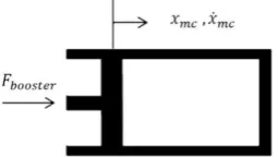
Fig. 4. The main cylinder model and exerted forced on it.
where 𝐴𝑚𝑐(𝑚2 ) is the main cylinder cross section, 𝐶𝑚𝑐(𝑁𝑚/𝑠) is the main cylinder damping coefficient, (N/m)𝐾𝑚𝑐 is the main cylinder spring stiffness, (𝐾𝑔)𝑀𝑚𝑐 is the main cylinder mass, 𝑃𝑚𝑐(𝑃𝑎) is the internal pressure within the main cylinder, and 𝑥𝑚𝑐 m is the piston displacement of the main cylinder.
(19)
𝑃𝑚𝑐= 𝛽𝑚𝑐
𝑉̇𝑚𝑐 𝑉𝑚𝑐
= 𝛽𝑚𝑐
𝐴𝑚𝑐𝑥̇𝑚𝑐− 𝑄𝑚𝑐+ 𝑄𝑤𝑜𝑢𝑡
𝑉𝑚𝑐
𝛽𝑚𝑐(𝑁/𝑚2 ) refers to the liquid bulk modulus, 𝑄𝑚𝑐(𝑚3/𝑠 ) to the oil flow rate discharged from the main cylinder, 𝑄𝑤𝑜𝑢𝑡 (𝑚3/𝑠) to the oil flow rate from the pump to the main cylinder, and 𝑉𝑚𝑐 (𝑚3) to the cylinder volume.
(20)
𝑄𝑚𝑐= 𝐶𝑚𝑐𝐶𝑑𝐴0×
√2 𝜌0
|𝑃𝑚𝑐− 𝑃𝑤𝑓𝑙− 𝑃𝑤𝑓𝑟− 𝑃𝑤𝑟𝑙− 𝑃𝑤𝑟𝑟| ×
sign(𝑃𝑚𝑐− 𝑃𝑤𝑓𝑙− 𝑃𝑤𝑓𝑟− 𝑃𝑤𝑟𝑙− 𝑃𝑤𝑟𝑟)
𝐶𝑚𝑐𝐶𝑑 refers to the main cylinder orifice discharge coefficient in terms of (𝑁𝑚/𝑠), 𝐴0(𝑚2) to the main cylinder exit cross section to the brake circuit, 𝜌0 (𝐾𝑔/𝑚3) to the oil density, and 𝑃𝑤(𝑓𝑙,𝑓𝑟,𝑟𝑙,𝑟𝑟) to the wheel cylinder pressure in terms of (𝑃𝑎).
3. Controller designing
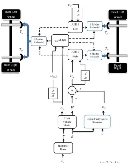
3. 1. The suggested structure for an anti lock-anti skid braking system
The suggested structure for an anti lock-anti skid braking system can be seen in Fig. 5, which consists of six fuzzy controllers, including four anti-lock and two anti-skid sub-controllers. In Fig. 5, three three-phase solenoid valves have been placed on the route of each wheel’s brake tubes, receiving commands from anti-lock and anti-skid controllers. As just mentioned, there are three phases to solenoid valves in this system.
In the first phase, the solenoid valve switches on, causing oil pressure to enter into each wheel’s brake circuit directly from the main cylinder.
In the second phase, the solenoid valve shuts off the brake tube, disconnecting the wheel brake circuit from the main cylinder. This prevents excessive brake pressure when the brake pedal is pressed.
In the third phase, the solenoid valve reduces the oil pressure within the wheel brake circuit to some extent.
The three stated phases are controlled by anti-lock and anti-skid controllers, with the first two phases pertaining to increase and decrease in (18)
𝐹𝑏𝑜𝑜𝑠𝑡𝑒𝑟− 𝐴𝑚𝑐𝑃𝑚𝑐− 𝐶𝑚𝑐𝑥̇𝑚𝑐− 𝐾𝑚𝑐𝑥𝑚𝑐
26
the anti-lock controller pressure, respectively, and the third phase being applicable in reducing brake torque through an anti-skid controller. In Fig. 5, the exerted force on the pedal and the steering angle applied by the driver are identified as system inputs.
The angular velocity of the wheels and its derivative (angular acceleration of each wheel) are utilized as inputs for anti-lock controllers. Yaw error angle, which is obtained by comparing the yaw angle with the desirable yaw angle, and its derivative are utilized as inputs for anti-skid controllers. The outputs for anti-lock and anti-skid controllers are control signals that examine the performance of solenoid valves. Furthermore, they prevent vehicles from locking up and being drifted away from the desirable path by controlling the hydraulic brake fluid flow into the wheels.
3. 2. Hydraulic brake anti-lock system
In this section, the fuzzy model and working principles of anti-lock controllers is discussed.
3. 2. 1. The working principles of anti-lock controllers
The purpose of the braking system is to reduce the braking time and distance, which is accomplished when the maximum friction coefficient between the wheel surface and that of the road is reached for. In addition to the friction coefficient, however, another factor, i.e. slip, is of significance in the braking process, and is defined as the Eq. (21).
(21) λ=𝑅𝑤𝜔𝑖− 𝑉𝑤𝑖cos (𝛼𝑖)
𝑉𝑤𝑖cos (𝛼𝑖)
; 𝑓𝑜𝑟 𝑖
= 𝑓𝑙, 𝑓𝑟, 𝑟𝑙, 𝑟𝑟
where λ is the amount of slip between the wheel and the earth, 𝑉𝑤𝑖cos (𝛼𝑖) is the wheel longitudinal velocity, 𝜔𝑖 is the angular velocity of each wheel, and 𝑅𝑤 is the wheel radius.
Fig. 5. anti lock (ALBS1) – anti skid (ASBS2) brake
system.
Upon braking, a difference is created in the speed of the wheel and that of the body, and the value of λ becomes restricted to a zero to -1 range. If wheels are locked up, then λ= −1. The wheel will experience a sharp deceleration just before getting locked up; if the wheel’s sharp deceleration process is not controlled it would get locked up before the required stoppage time for the vehicle has been passed. The controller will, then, increase the brake pressure for a second time until the sensor records a sharp reduction in speed. The controller does this task very rapidly before the wheel experiences a drastic change in speed. Consequently, the wheels will decelerate with the same speed rate as that of the vehicle, with the brakes keeping the wheels near the locking point, which allows for the maximum braking force to be applied in the system. Therefore, to prevent wheels from locking up during hard braking conditions, this controller needs to
JCARME Hydraulic anti-lock . . . Vol. 6, No. 1, Aut.-Win. 2016-17
27 create an increase as well as a decrease pressure
phase.
3. 2. 1. 1. Increase phase
In the increase phase, the oil flow reaches to the wheel cylinder directly from the main cylinder and through the solenoid valve, increasing the wheel cylinder pressure. In Fig. 6 the wheel brake circuit, including the wheel cylinder, brake pads, and wheel disks are illustrated. As is evident from the figure, the oil flow presses the wheel cylinder piston, which in turn presses the pad against the wheel disk, resulting in wheel deceleration and braking.
Fig. 6. the wheel brake circuit model.
Equations (22-25) are related to the wheel cylinder piston displacement in the increase phase [18], [19].
(22)
𝐴𝑤𝑃𝑤𝑓𝑙− 𝐹𝑤𝑓𝑙− 𝐶𝑤𝑥̇𝑤𝑓𝑙− 𝐾𝑤𝑥𝑤𝑓𝑙
= 𝑀𝑤𝑥̈𝑤𝑓𝑙
(23)
𝐴𝑤𝑃𝑤𝑓𝑟− 𝐹𝑤𝑓𝑟− 𝐶𝑤𝑥̇𝑤𝑓𝑟− 𝐾𝑤𝑥𝑤𝑓𝑟
= 𝑀𝑤𝑥̈𝑤𝑓𝑟
(24)
𝐴𝑤𝑃𝑤𝑟𝑙− 𝐹𝑤𝑟𝑙− 𝐶𝑤𝑥̇𝑤𝑟𝑙− 𝐾𝑤𝑥𝑤𝑟𝑙
= 𝑀𝑤𝑥̈𝑤𝑟𝑙
(25)
𝐴𝑤𝑃𝑤𝑟𝑟− 𝐹𝑤𝑟𝑟− 𝐶𝑤𝑥̇𝑤𝑟𝑟− 𝐾𝑤𝑥𝑤𝑟𝑟
= 𝑀𝑤𝑥̈𝑤𝑟𝑟
where 𝐴𝑤 (𝑚2) is the wheel cylinder cross section, 𝐶𝑤 (𝑁𝑚/𝑠) is the wheel cylinder damping coefficient, 𝐾𝑤 (𝑁/𝑚) is the wheel cylinder spring stiffness, 𝑀𝑤 (𝐾𝑔) the wheel cylinder mass, 𝑃𝑤(𝑓𝑙,𝑓𝑟,𝑟𝑙,𝑟𝑟)(𝑃𝑎) is the pressure exerted on the wheel cylinder, 𝐹𝑤(𝑓𝑙,𝑓𝑟,𝑟𝑙,𝑟𝑟)(𝑁) is the disc reaction force to
the wheel pad pressure, and 𝑥𝑤(𝑓𝑙,𝑓𝑟,𝑟𝑙,𝑟𝑟)(𝑚) is the wheel cylinder piston displacement in terms of 𝑚. Eqs. (26-29) are related to the generated pressure within four-wheel brake cylinders.
(26)
𝑃𝑤𝑓𝑙 = 𝛽𝑤
𝑉̇𝑤𝑓𝑙
𝑉𝑤𝑓𝑙
= 𝛽𝑤
𝑄𝑤𝑓𝑙− 𝐴𝑤𝑥̇𝑤𝑓𝑙
𝑉𝑤𝑓𝑙
(27)
𝑃𝑤𝑓𝑟 = 𝛽𝑤
𝑉̇𝑤𝑓𝑟
𝑉𝑤𝑓𝑟
= 𝛽𝑤
𝑄𝑤𝑓𝑟− 𝐴𝑤𝑥̇𝑤𝑓𝑟
𝑉𝑤𝑓𝑟
(28)
𝑃𝑤𝑟𝑙 = 𝛽𝑤
𝑉̇𝑤𝑟𝑙 𝑉𝑤𝑟𝑙
= 𝛽𝑤
𝑄𝑤𝑟𝑙− 𝐴𝑤𝑥̇𝑤𝑟𝑙 𝑉𝑤𝑟𝑙
(29)
𝑃𝑤𝑟𝑟= 𝛽𝑤
𝑉̇𝑤𝑟𝑟 𝑉𝑤𝑟𝑟
= 𝛽𝑤
𝑄𝑤𝑟𝑟− 𝐴𝑤𝑥̇𝑤𝑟𝑟
𝑉𝑤𝑟𝑟
where 𝛽𝑤(𝑁/𝑚2) is the liquid bulk modulus, 𝑄𝑤 (𝑚3/𝑠) is the oil flow rate in the wheel cylinder, and 𝑉𝑤 (𝑚3) is the main cylinder volume. According to Eq. (30), the flow rate input to each wheel cylinder is a quarter of the output flow from the main cylinder.
(30)
𝑄𝑤(𝑓𝑙,𝑓𝑟,𝑟𝑙,𝑟𝑟) = 1
4𝑄𝑚𝑐
3. 2. 1. 2. Decrease phase
In the decrease phase, the solenoid valve shuts off the oil flow route from the main cylinder to the wheel cylinder, causing the contained oil within the cylinder to be discharged, re-entering into the brake circuit through pumps. The solenoid valve remains in the decrease phase until the slip value is restored within the allowed range. Equations (31-34) are related to the wheel cylinder piston displacement in the decrease phase [18], [19].
(31)
𝐹𝑤𝑓𝑙− 𝐴𝑤𝑃𝑤𝑓𝑙− 𝐶𝑤𝑥̇𝑤𝑓𝑙− 𝐾𝑤𝑥𝑤𝑓𝑙
= 𝑀𝑤𝑥̈𝑤𝑓𝑙
(32)
𝐹𝑤𝑓𝑟− 𝐴𝑤𝑃𝑤𝑓𝑟− 𝐶𝑤𝑥̇𝑤𝑓𝑟− 𝐾𝑤𝑥𝑤𝑓𝑟
= 𝑀𝑤𝑥̈𝑤𝑓𝑟
(33)
𝐹𝑤𝑟𝑙− 𝐴𝑤𝑃𝑤𝑟𝑙− 𝐶𝑤𝑥̇𝑤𝑟𝑙− 𝐾𝑤𝑥𝑤𝑟𝑙
28
(34)
𝐹𝑤𝑟𝑟− 𝐴𝑤𝑃𝑤𝑟𝑟− 𝐶𝑤𝑥̇𝑤𝑟𝑟− 𝐾𝑤𝑥𝑤𝑟𝑟
= 𝑀𝑤𝑥̈𝑤𝑟𝑟
Due to the loss of oil pressure, and consequently the loss of brake torque in this phase, the disk reaction force pushes the pad back, resulting in oil discharge from the wheel cylinder. Equations (35-38) are related to the wheel cylinder pressure in the decrease phase.
(35)
Pwfl=βw
V̇wfl Vwfl
=βwAwẋwfl− Qwoutfl
Vwfl
(36)
𝑃𝑤𝑓𝑟= 𝛽𝑤
𝑉̇𝑤𝑓𝑟
𝑉𝑤𝑓𝑟
= 𝛽𝑤
𝐴𝑤𝑥̇𝑤𝑓𝑟− 𝑄𝑤𝑜𝑢𝑡𝑓𝑟
𝑉𝑤𝑓𝑟
(37)
𝑃𝑤𝑟𝑙 = 𝛽𝑤
𝑉̇𝑤𝑟𝑙 𝑉𝑤𝑟𝑙
= 𝛽𝑤
𝐴𝑤𝑥̇𝑤𝑟𝑙− 𝑄𝑤𝑜𝑢𝑡𝑟𝑙 𝑉𝑤𝑟𝑙
(38)
𝑃𝑤𝑟𝑟= 𝛽𝑤
𝑉̇𝑤𝑟𝑟 𝑉𝑤𝑟𝑟
= 𝛽𝑤
𝐴𝑤𝑥̇𝑤𝑟𝑟− 𝑄𝑤𝑜𝑢𝑡𝑟𝑟 𝑉𝑤𝑟𝑟
𝑄𝑤𝑜𝑢𝑡 is the oil flow discharged from the wheel cylinder, which is calculated from Eqs. (39-42).
(39)
𝑄𝑤𝑜𝑢𝑡𝑓𝑙= 𝐶𝑤𝐶𝑑𝐴0√ 2 𝜌0
|𝑃𝑤𝑓𝑙|𝑠𝑖𝑔𝑛(𝑃𝑤𝑓𝑙)
(40)
𝑄𝑤𝑜𝑢𝑡𝑓𝑟= 𝐶𝑤𝐶𝑑𝐴0√ 2 𝜌0
|𝑃𝑤𝑓𝑟|𝑠𝑖𝑔𝑛(𝑃𝑤𝑓𝑟)
(41)
𝑄𝑤𝑜𝑢𝑡𝑟𝑙 = 𝐶𝑤𝐶𝑑𝐴0√ 2 𝜌0
|𝑃𝑤𝑟𝑙|𝑠𝑖𝑔𝑛(𝑃𝑤𝑟𝑙)
(42)
𝑄𝑤𝑜𝑢𝑡𝑟𝑟 = 𝐶𝑤𝐶𝑑𝐴0√ 2 𝜌0
|𝑃𝑤𝑟𝑟|𝑠𝑖𝑔𝑛(𝑃𝑤𝑟𝑟)
Anti-lock fuzzy controllers have two inputs and an output. The first input is the difference between the angular velocity of each wheel and the average angular velocity of the three others at any given moment (∆ω). The second input is the angular acceleration of each wheel (a) and the controller output of the difference in pressure to the brake lining with normal pressure for braking without wheels to be locked. Fuzzy controller uses fuzzy rules and
changes the controller input to estimate the difference in pressure on the brake lining with ideal pressure and then ∆p = pideal− preal is calculated .To improve the accuracy of the control a range of ∆p is selected of the small fuzzy controller (shown between 10pa to -10 pa). On the way of the fuzzy output there is a switch that its output shows No. 1 in the case of a positive ∆p, otherwise, it shows 0. The switch opens and closes the flow of oil into the cylinder of the wheel brake, and when ∆p ≥ 0, it means that the pressure on the brake lining has not still reached the desired phase of braking pressure (output switch = 1); therefore, more pressure should be placed. When ∆p < 0, this means that the optimum braking pressure on the brake lining has increased and the risk of wheel locking has occurred. At this time, output is zero and phase of decreasing the pressure become activated. Therefore, output changes to a digital signal, on the verge of locking wheels. It causes the brake pressure in the wheel brake cylinders to be connected and disconnected. With the start of braking, acceleration and angular wheels will be negative and the range of zero to −40m
s2 for each wheel angular acceleration is intended as a proper control range (based on trial and error). Therefore, the range of 0 to −12m
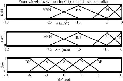
s is considered for an average speed difference of each wheel with the three others. In choosing interval fuzzy function, there are not the same range of spans. The more the velocity and the angular acceleration values are negative, the larger the interval fuzzy function is in order to precisely increase the control in determining the time of connecting and disconnecting the flow of oil braking in the wheels cylinder on the verge of wheels once they are to be locked. The membership functions and rules table for this controller are presented in Fig. 7 and Table 1, respectively.
3. 3. Hydraulic brake anti-skid system
JCARME Hydraulic anti-lock . . . Vol. 6, No. 1, Aut.-Win. 2016-17
29 3. 3. 1. The working principles of the controller
To prevent vehicle skid and yaw from the original path, the desirable path should, first, be estimated, and then vehicle yaw be prevented by comparing the actual motion path with the desirable motion path. To this end, the vehicle ideal yaw angle 𝜑𝑑 is first defined.
Fig. 7. Membership functions of anti-lock fuzzy controller inputs and output for front wheels.
Table 1. Anti-lock fuzzy controller rules table for front wheels.
3. 3. 1. 1. The vehicle ideal yaw angle
According to the stable spin theory, vehicle speed and yaw rate 𝑟 allow for Eqs. (43-46), [10-14].
(43)
𝐿 = 𝐿𝑓+ 𝐿𝑟
(44)
𝐴 = 𝑀𝑡
2𝐿2.
𝐿𝑟𝐶𝑦,𝑟− 𝐿𝑓𝐶𝑦,𝑓 𝐶𝑦,𝑟𝐶𝑦,𝑓
(45)
𝑟𝑑 =
1
1 + 𝐴𝑉2.
𝑉 𝐿. 𝛿
(46)
φ= ∫ 𝑟. 𝑑𝑡 , 𝜑𝑑= ∫ 𝑟𝑑. 𝑑𝑡
𝑡𝑒𝑛𝑑
𝑡𝑠𝑡𝑎𝑟𝑡
𝑡𝑒𝑛𝑑
𝑡𝑠𝑡𝑎𝑟𝑡
𝑟𝑑 is the vehicle desirable yaw rate, φ and φd are the vehicle ideal and actual yaw angles, respectively. 𝐶𝑦,𝑟 and 𝐶𝑦,𝑓 are lateral stiffness of the front and rear wheels, respectively. 𝑡𝑒𝑛𝑑 and 𝑡𝑠𝑡𝑎𝑟𝑡 are the starting and end times of braking, respectively, and 𝑉 is the vehicle body speed. In vehicles without any controller, wheels change much more rapidly in speed than bodies do, in hard braking conditions. Therefore, the body speed would not be measurable in such situations. However, by preventing the wheel speed from experiencing sudden changes, and subsequently from locking up, anti-lock brakes bring wheel and body speed changes closer to each other in braking situations. It could be stated, therefore, that according to Eq. (47), the body speed is approximately equal to the average linear speed of the four wheels.
(47)
𝑉 = 𝑅𝑤(𝜔𝑓𝑙+ 𝜔𝑓𝑟+ 𝜔𝑟𝑙+ 𝜔𝑟𝑟)/4
Braking on roads with various friction coefficients, and hard braking situations on road twists are among the most important situations in which vehicles are exposed to skids. At the time of braking, detour occurs when the vehicle brake torque of the sides are not equal. When the two sides of the vehicle wheels experience different friction coefficients, brake torque difference between the side wheels is created. The wheel, which is located on the slippery side has lower braking torque than the other wheels. It should be considered that anti-skid controller finds wheels with high friction coefficient and reduces the braking torque to balance between the torque of the wheels on the car sides by checking the control inputs and identifying the detour of cars. Anti-skid Mamdani type fuzzy controllers have two control inputs: ∆𝜑 = 𝜑𝑑− 𝜑 which refers to the vehicle yaw angle from the desirable trajectory, and 𝑑(∆𝜑)/𝑑𝑡 which refers to the vehicle yaw rate. The fuzzy controller output, i.e. 𝐾, controls the brake fluid flow rate into the wheel brake pad. If the inputs’
-40 -25 -15 -5 0
0 1
a (m/s2)
D
oM VBN BN N Z
Front wheels fuzzy memberships of anti lock controller
-12 -7.5 -4.5 -1.5 0
0 1
(m/s)
D
oM VBN BN N Z
-10 -6 -3 0 3 6 10
0 1
P (pa)
D
oM BN N Z P BP
Z N
BN VBN
∆𝜔 𝑎
P Z
N BN
VBN
BP P
Z N
BN
BP BP
P Z
N
BP BP
BP P
30
changes are insignificant, then = 0, meaning that the controller allows the brake fluid flow to completely penetrate into the brake pad. Otherwise, if the amounts of inputs increase more than a certain extent, would have a value in the range of 0 – 1. The input oil flow rate to the wheel cylinder is proportional to the value of . For instance, if = 0.25, only 3 4 of the input oil flow would enter into the wheel cylinder. The membership functions and rules table for this controller are presented in Fig. 8 and Table 2, respectively.
In designing anti-skid controllers, an important point is to use an appropriate control input not only to assist in the timely identification of vehicle yaw but to display resistance against rapid changes of road conditions. For instance, if placed on a road, which is initially only slippery on the right-hand side and suddenly the road situation is reversed, i.e. it is only slippery on the left-hand side, and the input should be able to properly identify these rapid changes in road conditions. Therefore, in the simulations conducted in section four, the impact of two inputs, namely, yaw angle and yaw rate, on the controller performance under rapid road condition changes is examined. To achieve this, an anti-skid controller with angle yaw as control input together with its derivative is, first, used, and the process is repeated for the yaw rate as the other control input.
4. Simulation
In this section, each of anti-lock and anti-skid controllers is examined under different maneuvers. The simulations were conducted under MATLAB/Simulink environment. It should be noted that the vehicle initial speed was deemed 120 km/h for all presented maneuvers.
4. 1. The evaluation of anti-lock controller performance
Anti-lock controllers are expected to prevent wheels from locking up when their speed decelerates more rapidly than that of the vehicle; thus assisting drivers in better handling
of vehicles by reducing the braking distance. The performance of an anti-lock controller was studied on a dry-asphalt road, with the friction coefficient of = 1, a zero steering angle, and a brake pedal force as illustrated in Fig. 9. The wheel slip curve with/without using an anti-lock controller and the exerted brake torque wheel with/without using an anti-lock controller are demonstrated in Fig. 10 and 11, respectively. The braking time and the driver’s reaction time for pushing and releasing the brake pedal were assumed 2 and 0.1 seconds, respectively.
Fig. 8. Membership functions of anti-skid fuzzy
controller inputs and output for left wheels.
Table 2. Anti-skid fuzzy controller rules table for
left wheels.
VBP BP
P Z
∆
∆
PM PS
Z Z
Z
PB PM
PS Z
P
PVB PB
PM PS
BP
PVB PVB
PB PM
VBP
Fig. 9. The exerted force on the brake pedal.
0 0.15 0.3 0.5
0 1
(rad)
D
oM Z P BP VBP
Left wheels fuzzy memberships of anti skid controller
0 0.15 0.3 0.5
0 1
d()/dt (rad/s)
D
o
M Z P BP VBP
0 0.3 0.55 0.75 0.9 1
0 1
Kleft
D
o
M Z PS PM PB PVB
0 0.1 2.12.2
0 32
t (s)
F
p
(N
)
JCARME Hydraulic anti-lock . . . Vol. 6, No. 1, Aut.-Win. 2016-17
31 As can be seen from Fig. 10 and 11, on hard
braking conditions with a 32-newton brake pedal force and without using an anti-lock controller, the wheels locked up within less than the first second of braking. Through the proper shutting off and releasing of the braking torque in front and rear wheels, and by maintaining the wheel slip value within the range of −0.3 ≤λ≤ −0.2, the anti-lock controller prevented the wheels from locking up and the vehicle from yawing, which resulted in a reduced braking distance. Note that the cause of the difference between the curves of the front and rear wheel skid is the difference in the force of weight to the wheels. At the time of braking, the vehicle weight is on the front wheels and therefore front wheels experience friction. Consequently, skid of the rear wheels will be larger.
Fig. 10. The wheels slip curves with/without using an anti-lock controller.
4. 2. The evaluation of anti-skid controller performance
The anti-skid controller performance should be evaluated alongside its anti-lock counterpart, in that, in case the wheels get locked up, the anti-skid controller would no longer be capable of preventing vehicle yaw. As a complement to the anti-lock controller, the anti-skid controller plays a fundamental role in vehicle control
under critical conditions, such as roads with different coefficients of friction, hard braking situations on road twists, and maneuvers that include multiple direction changes. The controller performance with respect to maintaining the intended vehicle trajectory could be analyzed and evaluated by simulating any of such scenarios.
Fig. 11. The wheels torque curves with/without using an anti-lock controller.
4. 2. 1. Roads with different coefficients of friction
In this section, the controller performance is evaluated by assuming a zero steering angle and four specified situations in A-D. It is worth noting that the specified situations are consistent throughout the braking process. Braking [takes place] on a normal road with 𝜇𝑝𝑒𝑎𝑘 = 1 without utilizing any controller; the vehicle trajectory in this situation is taken as the reference trajectory.
Braking on a road with 𝜇𝑝𝑒𝑎𝑘= 1 for left wheels and 𝜇𝑝𝑒𝑎𝑘= 0.7 for right wheels, without utilizing any controller.
0 0.9 1.4 2.1
-1 0
t (s)
Slip curve without using controller
Front wheels Rear wheels
End of braking
0 0.1 2.1
-0.3 -0.2 0
t (s)
Slip curve using only anti lock controller
Front wheels Rear wheels
End of braking
0 0.1 2.1
-715 0
Braking torque without using controller
t (s)
(N
.m
)
0 0.1 2.1
-715 0
t (s)
(N
.m
)
Braking torque of front wheels
0 0.1 2.1
-715 0
t (s)
(N
.m
)
32
Braking on a road with 𝜇𝑝𝑒𝑎𝑘= 1 for left wheels and 𝜇𝑝𝑒𝑎𝑘= 0.7 for right wheels, using merely a single anti-lock controller.
Braking on a road with 𝜇𝑝𝑒𝑎𝑘= 1 for left wheels and 𝜇𝑝𝑒𝑎𝑘= 0.7 for right wheels, using anti-lock and anti-skid controllers (with yaw angle as control input)
Assuming pedal force, an approximate of about 16 Nm simulations of the above situations is done. As seen in Fig. 12, the steering angle in all the maneuvers is zero, the only factor of the vehicle's yaw is the road conditions. Considering the mentioned conditions in every single maneuver, the first one indicates the car is moving in a straight line. In the second one, the vehicle (difference in coefficient of friction of the two sides of the vehicle) is skidded and distracted due to road conditions. In the third one, the anti-lock controller only prevents wheels to be locked, but when the wheels do not lock it can also skid due to the road conditions. Hence, anti-lock controller is an important but not sufficient factor to control the vehicle. At last, in the last situation, anti-lock/skid controllers help the vehicle to go in the right direction.
Fig. 12. The vehicle trajectory with/without using a controller.
Another undesirable condition during driving is friction coefficient changes that could take place during the braking time. Therefore, the previous maneuver is repeated using the friction coefficient of Fig. 13.
Fig. 13. Friction coefficient changes in left and right wheels during braking.
Figure 14 demonstrates that the anti-lock controller was not capable of preventing vehicle yaw. In contrast to the previous maneuver, the anti-skid controller with an input control of yaw angle was not able to fully maintain the vehicle balance along the desirable trajectory due to changes in friction coefficients during braking. To explain the above point, it is sufficient to review Eqs. (45 and 46) from the third section. As can be seen, yaw angle is calculated from the integration of the vehicle yaw rate. Among the integrator’s deficiencies is its prolonged settling time, in that, the integrator cannot estimate the yaw angle in a precise and speedy manner with rapid condition changes. Consequently, the controller cannot operate in a precise manner, and the vehicle is rendered incapable of moving along the desirable trajectory. The provided descriptions, as well as the obtained simulation, results from Fig. 15 point to a superior maintenance of vehicle trajectory when using a yaw rate as a control input.
Fig. 14. Vehicle trajectory on a road with different friction coefficients with/without the controller.
0 60
-5 0
x (m)
y
(m
)
Vehicle lane during braking on slippery road
Using anti lock-anti skid controller
Without any controller Using only anti lock Reference lane
0 2.1
0.5 1
t(s) r
Friction coefficient curve of left and right wheels
0 2.1
0.5 1
t(s) l
End of braking End of braking
0 80
-7 0
x(m)
y(
m
)
Vehicle lane during braking on -split road
JCARME Hydraulic anti-lock . . . Vol. 6, No. 1, Aut.-Win. 2016-17
33
Fig. 15. Comparing the performance of anti-skid controller in use of yaw angle and yaw rate.
4. 2. 2. Hard braking situations on road twists
Another critical condition is hard braking on road twists. In this section, the anti-skid controller performance is evaluated by conducting a single-redirect, as well as double-redirect maneuvers.
4-2-2-1. Single-redirect maneuvers
The following four maneuvers were simulated by applying a fixed steering angle to the vehicle with 𝜇𝑝𝑒𝑎𝑘 = 1 on a dry-asphalt road.
a) Braking with an 18-newton pedal force and a 10-dgeree steering angle, without utilizing any controller.
b) Braking with a 32-newton pedal force and a 10-degree steering angle, without utilizing any controller.
c) Braking with a 32-newton pedal force and a 10-degree steering angle, using anti-lock controller.
d) Braking with a 32-newton pedal force and a 10-degree steering angle, using anti lock-anti skid controller (with yaw angle as control input).
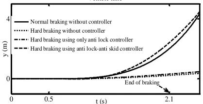
Based on Fig. 16, a soft braking (maneuver A) during a vehicle turn would not lead to any difficulties. Yet, doing the same maneuver with a more intense breaking force (maneuver B) deprives the vehicle of a proper turn, resulting in a phenomenon known as understeer due to locking up the front wheels. As can be seen, anti-lock controller, too, is not capable of improving such situation (maneuver C). However, anti lock-anti skid controller (maneuver D) allows for a proper handling of vehicle and the application of an appropriate steering angle.
Fig. 16. Comparing normal and hard brakings on road twists with/without using a controller.
In Fig. 17, the curve for wheel braking torque changes is illustrated. The desirable performance of controllers in different moments during braking is evident. As can be seen, despite a similar friction coefficient on the part of the wheels, anti-skid controller was more active in left wheels as a result of a left-hand turn and the subsequent state of slipperiness experienced by left wheels. Anti-lock controller was more active in the front right wheel. In rear wheels, both anti-lock and anti-skid controllers functioned during different times, based on the wheel speed and the vehicle yaw rate.
Fig. 17. Wheels torque curves upon braking during turning left.
4. 2. 2. 2. Double-redirect maneuvers
By applying the steering angle in Fig. 18 on a dry-asphalt road and with 𝜇𝑝𝑒𝑎𝑘= 1 , the following four maneuvers were simulated. Braking with an 8-newton pedal force, without utilizing any controller (the reference trajectory).
0 80
-0.1 -0.03 0.1 0.35
x(m)
y(
m
)
Comparing the performance of anti skid controller in use of yaw angle and yaw rate
Reference lane Using yaw angle control Using yaw rate control
0 0.5 2.1
0 4
t (s)
y
(m
)
Vehicle lane
Normal braking without controller Hard braking without controller Hard braking using only anti lock controller Hard braking using anti lock-anti skid controller
End of braking
0 2.1
-1000 0
t(s)
fl
(N
.m
)
Braking torque of each wheel
0 2.1
-1000 0
t(s)
fr
(N
.m
)
0 2.1
-1000 0
t(s)
rl
(N
.m
)
0 2.1
-1000 0
t(s)
rr
(N
.m
34
Braking with an 18-newton pedal force, without utilizing any controller.
Braking with an 18-newton pedal force, using anti lock-anti-skid controller (with yaw angle as control input).
Braking with an 18-newton pedal force, using anti lock-anti-skid controller (with yaw rate as control input).
The vehicle overall maneuverability is reduced in above speeds, rendering the application of an acute steering angle impossible. As can be seen from Fig. 19, the vehicle was capable of handling a 10-degree steering angle under extremely soft braking conditions, i.e. an 8-newton pedal force. However, should the pedal force increase, not only the vehicle cannot maintain the intended trajectory, but it can lead to vehicle yaw or even overturn. A great vehicle yaw and an eventual overturn for an 18-newton pedal force can be observed. Anti-skid controller with a yaw angle control input improves vehicle trajectory to a great extent, and the performance of an anti-skid controller would be even more enhanced by using a yaw rate control input, drawing the vehicle trajectory nearer to that of the reference. Taking the conducted simulations into account, it is suggested that yaw rate is used in place of yaw angle as control input in anti-skid controllers.
Fig. 18. The steering angle applied to the vehicle.
Fig. 19. The vehicle trajectory during double redirects.
5. Conclusions
Wheel and body simulation with seven degrees of freedom, modeling the vehicle dynamic motion, as well as modeling all parts within a hydraulic braking system, including pedal, the main brake cylinder, wheel brake cylinders, and even modeling the driver’s foot pressure on the pedal, allowed for a carefully studying and a reliable designing of an intelligent brake system. This is claimed as one of the strengths of this article compared to other studies. The conducted simulations demonstrate the desirable performance of anti-lock controllers in reducing braking time and distance under hard braking situations. There are two ways to estimate the operation of controllers: a) making a mechanical system and comparing the results with those practical ones that it both takes time and money, or b) examining the controller’s operation in critical driving conditions. In a normal situation, it is expected that the vehicle goes without skidding or wheels to be locked. However, the wheels are locked or the vehicle skids, if the friction coefficient reduces on one side of it or a strong braking in the roads curve happens, and its wheels is locked and the controller can manage this condition. The better examination of a controller is when there is an even worse critical condition. Therefore, in stimulation for preparing this paper, the assumption of the sudden reduction of the friction coefficiency of one side of the vehicle or braking with more force on the roads curve makes the condition the best way to estimate the controller. Regarding the performance of anti-skid controllers in maneuvers that do not contain rapid condition changes, it was revealed that it operates favorably with a yaw angle control input. Yet, in maneuvers in which it was faced with rapid condition changes, the yaw angle follows rapid changes with a delay due to prolonged settling time on the part of an integrator (see equations from section 3-3-1-1). Such delay introduced errors in the vehicle trajectory compared to the desirable path. This issue is resolved in controllers with yaw rate control inputs due to a lack of need for an integrator.
0 0.5 1.5 2.5 3 3.5 4.5
-10 0 10
t(s)
(d
eg)
Steering angle applied to the vehicle
0 120
0 30
x(m)
y(
m
)
Vehicle lane during double redirects
JCARME Hydraulic anti-lock . . . Vol. 6, No. 1, Aut.-Win. 2016-17
35
References
[1] M. J. Gutnecht, D. R. Schniedewend, J. J. Moskwa, C. R. kime and P. Romanathan, "Fault tolerance analysis of alternate automative brake system designs", SAE Technical paper, No. 930511, (1993).
[2] R. H. Madison and H. E. Riordan, "Evolution of the sure track brake system", SAE Technical paper, No. 690213, (1969).
[3] C. Orthwein , "Clutches and brackes design and selection" , Marcel Dekker Inc., chapter 12, (2004).
[4] N. Patra and K. Datta, " Improved sliding mode controller for anti- lock braking system", In Proc. CALCON11, pp. 25-30, Kolkata, Nov., (2011).
[5] A. Harifi, A. Aghagolzadeh, G. Alizadeh, M. Sadeghi, "Designing a sliding mode controller for slip control of antilock brake system", Transportation Research Part C, Vol. 16, pp. 731-741, (2008). [6] C. Edwards and S. spurgeon, “"Sliding
mode control: Theory and applications", London, UK: Taylor and francis, (1998). [7] V. Utkin, Sliding modes in control and
optimization, USA: Springer- Verlag, Berlin, (1992).
[8] Y. Tang, X. Zhang, D. Zhang, G. Zhao and X. Guan, "Fractional order sliding mode controller design for antilock braking systems" Jornal of Neurocomputing, Vol. 111, pp. 122-130, (2013).
[9] N. Patra and k. Datta , " Sliding mode controller for wheel–slip control of anti-lock braking system", Proceedings of the Advanced Communication Control and Computing Technologies Conference, pp. 385-391, Rourkela, India, 23-25 August, (2012).
[10] P. Naderi, S. M. T. Bathaee and A. farhadi, "Driving/regeneration and stability enhancement for a four-wheel-drive hybrid vehicle", International Review of Electrical Engineering, Vol. 4, No. 1, (2009)a.
[11] P. Naderi, M. Mirsalim and S. M. T Bathaee, "Driving/regeneration and stability enhancement for a two-wheel-drive electric vehicle", International Review of Electrical Engineering, Vol. 4, No. 1, (2009)b.
[12] P. Naderi , A. R. Naderipoar, M. Mirsalim and M. A. fard, "Intelligent braking system using fuzzy logic and sliding mode controller", Jornal of Control and Intelligent Systems, Vol. 38, No. 4, pp. 236-244, (2010).
[13] P. Naderi and A. Farhadi, "Non-driven wheels application for intelligent multi-objective control of hibrid vehicles", International Journal of Robotics and Automation, Vol. 27, No. 2, pp. 185-197, (2012).
[14] W. Xiany, P. C. Richardson, C. Zhao and S. Mohammad, "Brake-by-wire control system design and analysis", IEE Transaction On Vehicular Technology, Vol. 57, No. 1, PP. 138-147, (2008). [15] P. Naderi and S. M. sharouni, "Intelligent
braking system for stability enhancement of vehicle braking, using fuzzy logic controllers", International Jornal of Vehicle Safety, Vol. 6, No. 4, PP. 381-398, (2013).
[16] V. C´irovic´and D. Aleksendric´, "Adaptive neuro-fuzzy wheel slip control", Jornal of Expert Systems with Applications, Vol. 40, pp. 5197-5209, (2013).
[17] R.-E. Precup, et al., "Nature-inspired optimal tuning of input membership functions of takagi-sugeno-kang fuzzy models for anti-lock braking systems", Appl. Soft Comput. J. (2014).
[18] M. Wu and M. shih , "Simulated and experimental study of hydranlic anti-lock braking system using sliding mode PWM control" Jornal of Mechatronics,Vol. 13, No. 4, pp. 331-351, (2001).
36
[20] J. H. park, D. H. Kim and Y. J. Kim, "Anti-lock brake system control for buses based on fuzzy logic and a sliding-mode observer ", International Jornal of KSME, Vol. 15, No. 10, pp. 1398-1407, (2001).
[21] H. Lin and Ch. Song, "Simulation of hydraulic anti-lock braking system control based on a co-simulation model by AME sim and simulink", Proceedings of TMEE Conference, pp. 775-778, Changchun, China, 16-18 December (2011).
[22] M. Kato, T. Matsuto, K. Tanaka, H. Ishihara and W. Hosoda, "Combination of anti-lock brake system (ABS) and combined brake system (CBS) for motorcycles", SAE. 960960, pp. 1284-129, (1996).
[23] A. Strichland and K. Dagg, "ABS braking performance and steering input", SAE Special Publications, 980240, pp. 57-64, (1998).
[24] F. M. Georg, F. G. Gerard and C. Yann, "Fuzzy logic continuous and quantizing control of an ABS braking system", SAE. 940830, pp. 1033-1042, (1994).
[25] N. Miyasaki, M. Fukumoto, Y. Sogo and H. Tsukinoki, "Anti-lock brake system (M-ABS) based on the friction coefficient between the wheel and the
road surface", SAE special publications, 900207, pp.101-109, (1990).
[26] C. Y. Lu and M. C. shih "Application of the pacejka magic formula tyre model on a study of a hydraulic anti-lock braking system for a light motorcycle", Vehicle System Dynamics, Vol. 6, No. 41, pp. 431-448, (2004).
[27] M. Sugai, H. Yamaguchi, M. Miyashita, T. Umeno and K. Asano , "new control technique for maximizing braking force on anti- lock braking system", Vehicle System Dynamics, No. 32, pp. 229-312, (1999).
[28] Ch. K. Huang and M. Ch. Shih , "Design of a hydraulic anti–lock braking system (ABS) for a motorcycle", Journal of Mechanical Science and Technology, Vol. 5, No. 24, pp. 1141-1149, (2010). [29] B. Wang, et al., "a Robust wheel slip
ratio control design combining hydraulic and regenerative braking systems for in-wheel-motors-driven electric vehicles", Journal of the Franklin Institute, (2014). [30] H. Mirzaeinejad, M. Mirzaei,
"Optimization of nonlinear control strategy for anti-lock braking system with improvement of vehicle directional stability on μ -split roads", Jornal of Transportation Research Part C, Vol. 46, pp. 1-15, (2014).
Attachments
The simulated vehicle’s specifications.
Amount Unit
Symbol Definition
1027
𝐾𝑔/𝑚3 𝜌0
Brake fluid density
1.2 × 10⁻⁸ 𝑚2
𝐴0
The maximum cross section of oil tubes
6.9 × 10⁵ 𝑁/𝑚2
β
Liquid bulk modulus
2.85 × 10⁻⁴ 𝑚2
𝐴𝑚𝑐
The main cylinder cross section
100
𝑁𝑚/𝑠 𝐶
Damping coefficient
1.8 × 10⁻⁴ 𝑚2
𝐴𝑤
Wheel cylinder cross section
2.85 × 10⁻⁷ 𝑚3
𝑉𝑚𝑐0
The main cylinder initial volume
5.4 × 10⁻⁷ 𝑚3
𝑉𝑤0
Wheel cylinder initial volume
50
𝑁⁄𝑚 K
Cylinder spring stiffness
0.001 _
_
𝐶𝑑
Orifice coefficient
1027
𝐾𝑔/𝑚3 𝜌0
Brake oil coefficient
1.2 × 10⁻⁸ 𝑚2
𝐴0
JCARME Hydraulic anti-lock . . . Vol. 6, No. 1, Aut.-Win. 2016-17
37 6.9 × 10⁵
𝑁/𝑚2 β
Liquid bulk modulus
2.85 × 10⁻⁴ 𝑚2
𝐴𝑚𝑐
The cross section of the master cylinder
100
𝑁𝑚/𝑠 𝐶
Damping coefficient
1.8 × 10⁻⁴ 𝑚2
𝐴𝑤
The cross section of the wheel cylinder
2.85 × 10⁻⁷ 𝑚3
𝑉𝑚𝑐0
The initial volume of the main cylinders
50
𝑁⁄𝑚 K
Cylinder spring stiffness
0.001 _
_
𝐶𝑑
Damping coefficien
850 kg
𝑀𝑡
Vehicle’s total mass
1.147 m
𝐿𝑓
The distance from the front axis to the center of gravity
1.197 m
𝐿𝑟
The distance from the rear axis to the center of gravity
1800
𝐾𝑔. 𝑚2 𝐼𝑧
Vehicle inertia around the z-axis
17500 N
𝐶𝑥
Wheel longitudinal stiffness
15000
𝑁 𝑟𝑎𝑑 ⁄ 𝐶𝑦
Wheel lateral stiffness
0.5 m
ℎ𝑐𝑔
The center of gravity height
1.4 m
𝑇𝑎
The length of vehicle axes
0.275 m
𝑅𝑤
The wheel radius
3.2639
𝐾𝑔. 𝑚2 𝐼𝑤