NGARCH MODEL AS AN ALTERNATIVE TO THE
BLACK-SCHOLES MODEL
Petra POSEDEL, MSc Professional article*
Faculty of Economic and Business, Zagreb UDC 336.748(497.5)
JEL C21
Abstract
The interest of professional investors in financial derivatives on the Croatian market is steadily increasing and trading is expected to start after the establishment of the legal framework. The quantification of the fair price of such financial instruments is therefore becoming increasingly important. Once the derivatives market is formed, the use of the Black-Scholes option pricing model is also expected. However, contrary to the assump-tions of the Black-Scholes model, research in the field of option markets worldwide sug-gests that the volatility of the time-series returns is not constant over time. The present study analyzes the implications of volatility that changes over time for option pricing. The nonlinear-in-mean asymmetric GARCH model that reflects asymmetry in the distri-bution of returns and the correlation between returns and variance is recommended. For the purpose of illustration, we use the NGARCH model for the pricing of foreign currency options. Possible prices for such options having different strikes and maturities are then determined using Monte Carlo simulations. The improvement provided by the NGARCH model is that the option price is a function of the risk premium embedded in the under-lying asset. This contrasts with the standard preference-free option pricing result that is obtained in the Black-Scholes model.
Key words: Black-Scholes model, NGARCH model, heteroscedasticity, volatility, risk premium, risk-neutral measure, no arbitrage, Monte Carlo simulations.
1 Introduction
An explosive increase in trading with different financial instruments on the Croatian market inspires and motivates us to model prices of various assets, foreign currency and exchange rates and their volatilities. So far, trading with derivatives on the Croatian market is only of over-the-counter (OTC) type. The Croatian market for nonlinear derivatives-options does not exist yet, but the possibility of its being formed attracts the interest of many investors on the Croatian capital market. It is, thus, of increasing importance to quantify the fair price of such objects. We can not focus our research on data from options markets because these do not exist yet. Since the debate on whether to introduce a derivatives market is still open, this work tries to make another contribution on possible prices of European call options for assets. First of all, such a goal requires an appropriate econometric modelling of price dynamics of assets and their volatilities since option pricing formulas are functions of some or all parameters present in the model describing the price dynamics of assets. One of the great successes of modern financial economics is option pricing. Based on the well-known Law of One Price or no-arbitrage condition, the option pricing models of Black and Scholes (1973) and Merton (1973) gained an almost immediate acceptance among academics and investment professionals of a kind unparalleled in the history of economic science.1
However, contrary to the assumptions of the Black-Scholes model, research in the field of option markets worldwide (e. g. Mandelbrot (1963) and Fama (1965) in their works base their empirical studies on log-returns of several US stocks) suggest that the volatility of time series returns is not constant over time. In fact, during stress periods
on the market (political changes or disorders, economic crises, but also not so drastic changes like announcements of macroeconomics data) prices of financial assets fluctuate very much and the volatility changes over time. In this case we say that the process of interest is heteroscedastic. The first plausible success of econometrical modelling of the heteroscedasticity of time series is attributed to Engle (1982) who introduced the ARCH model. Various extensions of the ARCH model were subsequently made by many researchers. Bollerslev (1986) and Taylor (1986), independently of each other, suggested the generalized ARCH, i.e. the GARCH model, and Nelson (1991) the exponential GARCH, i.e. the EGARCH model. The leverage effect and other GARCH extensions are described in the works of Ding, Granger and Engle (1993), Glosten, Jagannathan and Runkle (1993) and Hentschel (1995). Bollerslev, Chou and Kroner (1992) and the work of Duan (1997) encompassed the existing GARCH models into a common system known as the augmented GARCH (p,q) process.
On the Croatian market, Šestović and Latković applied the GARCH (1,1) model for analyzing stocks of PLI-AA, ZAB-O and of the CROBEX index. The authors conclude that using models from the GARCH family improves predictions of market risk.
heteroscedasticity can reflect changes in the conditional variance of assets. Furthermore, the numeric analysis in these works suggests that the proposed models can potentially explain some well-documented systematic biases associated with the Black-Scholes model, like underpricing of out-of-the-money options.
We ask if the situation regarding pricing foreign currency options is somehow similar to pricing equity options? Cooper et al. (1986) estimate the parameters of the stochastic process describing changes in volatilities and compare the predicted prices to Black-Scholes prices afterwards. Their results are similar in nature to those found in studies on stock options.
Prices in option markets are commonly quoted in terms of the Black-Scholes implied volatility. In Rebonato’s terms (1999), the implied volatility is a “wrong number which, plugged into the wrong formula, gives the right answer!” This does not mean that market participants believe in the hypotheses of the Black-Scholes model – they do not: the Black-Scholes formula is not used as a pricing model for vanilla options but as a tool for
translating market prices into a representation in terms of implied volatility.
The interest of participants on the Croatian market have been lately attracted by interventions of the Croatian National Bank on the domestic market resulting in changing the market value of the domestic currency. Seasonality trends typical for domestic currency and the possibility of changing the domestic currency in the future motivate us to explore different kinds of foreign currency options, with different strikes and maturities. The goal of this work is to analyze the empirical distribution of the EUR/HRK currency time series and the consequences that such analysis has for pricing foreign currency options. The primary goal of this study is to estimate the parameters appearing in the dynamics of the currency time series using the nonlinear-in-mean, asymmetric GARCH model. The obtained parameters are then used for simulating prices of foreign currency options implementing the NGARCH option pricing model. Furthermore, we compare the obtained prices with the Black-Scholes ones. The following addressed issue is to explore if the heteroscedasticity assumption for changes in the time series present in the NGARCH model reflects visible differences in option prices. Doing this we are trying to connect the very popular econometric GARCH model and the literature all over about contingent claims.
The article is organized as follows. In the second part of the work we introduce the non linear asymmetric GARCH model for describing the EUR/HRK currency dynamics for short time horizons in the period 2001-2005, we describe the properties of the model and estimate the parameters. Option pricing in the NGARCH framework is presented in the third part. Option prices for foreign currency implementing the NGARCH model and the analysis among different strikes and maturities are described in the fourth part and compared to prices derived from the constant volatility model of Black and Scholes. In the conclusion we address future issues and research.
2 Modelling the exchange rate with the NGARCH model
values for investors are log-returns,2 i.e. the differences in the closing prices during a one day period,
Pt+1=lnCt+1−lnCt. (1)
Figure 1 compares increments of a Brownian motion with the returns on the EUR/ HRK exchange rate with the same average volatility. While both return series have the same variance, the Brownian model achieves it by generating returns which always have roughly the same amplitude and manifest frequent large peaks representing some unexpected change on the market.
Figure 1 Daily log-returns for the EUR/HRK exchange rate
0.018
0.010
0.000
-0.010
-0.018
2/1/2001 2002 2003 2004 2005 30/12/2005
0.018
0.010
0.000
-0.010
-0.018
0 300 600 900 1.297
Number of simulated returns
Note: (Top) compared to the log-returns of the Blach-Scholes model (bottom) with same annuali-zed mean and variance
A lot of empirical research indicates the increasing need for a more realistic model for financial assets than the Brownian one. Experience has shown that returns volatility for most financial instruments is not constant over time. Rather, days of high (low) volatilities are followed by days of high (low) volatilities, a property known as clustering. For the purpose of estimating the variability of returns, the variable representing the squared innovation return is of crucial importance,
St Pt E Pt
2 2
= ( −μ) , μ= ( ). (2)
Figure 2 describes the changes in the EUR/HRK exchange rate prices in the period from 2001 to 2005. It can be immediately noticed that some periods have very different volatilities, which can be also seen from the graph of the squared innovation returns.
Figure 2 The dynamics of the EUR/HRK exchange rate and squared innovations in the period 2001-2005
7.8
7.6
7.4
7.2
7
2/1/2001 2002 2003 2004 2005 30/12/2005
4
3
2
1
0
2/1/2001 31/12/2005
x104
autocorrelations of squared daily returns have positive values for small lags and then go exponentially to zero when the number of lags increases. This shows that squared returns values do not forget the recent past and that they are positively correlated which can be seen from the dotted line in figure 3.
At first glance it may perhaps seem that the problem of pricing call options is solved by the use of the standard Black-Scholes formula, where we use domestic rate rd as the
short rate of interest, and the stock price C is replaced by the exchange rate. This line of argument is, however, incorrect and the reason is as follows. When we buy a stock (without dividends) we, in principle, buy a piece of paper which we keep until we sell it. On the other hand, when we buy a foreign currency we will, on the contrary, not just keep the physical currency bills until we sell them again. Instead we will typically put the currency into an account where they will grow at a certain rate of interest. The obvious implication of this fact is that a foreign currency plays very much the same role as a domestic stock with a continuous dividend. Thus, modelling foreign currency requires the introduction of the foreign interest rate in standard models for stocks that will play an important role in pricing currency options.
2.1 Description of the model
Suppose we are observing the discrete economy and denote with Ct the EUR/HRK
exchange rate price in time t, defined as the number of Croatian kunas required to purchase one euro. The dynamics of the time series of return Pt is described with a
nonlinear-in-mean, asymmetric GARCH (1,1)3 model (Engle and Ng, 1993):
P C
C r r Z
t
t t
d s t t t t
+1≡ +1 − + +1− +1+ + +
2 1
( ) = 1
2
ln λσ σ σ 11, (3)
σt2+1=ω α σ+ ( tZt−ρσt)2+βσt2, (4)
where Zt are i.i.d. standard normal random variables N (0,1) and
ω> 0, α ≥0, β≥0 and α(1+ρ2)+β< (5)
in order to insure the non negativity and stationarity of the variance process σ2
t. Variables rd and rs denote, respectively, the constant one period riskless domestic and foreign interest
rate,4 while λ is the constant risk premium, i.e. the reward for investing in the foreign currency. The value of the premium will influence the conditional variance of the process
3It is worthwhile to mention that very often in literature the asymmetric GARCH model is called NGARCH.
4In this work, for illustration purposes, r
d and rs are taken as constants of known values. It is possible to
when doing option pricing.5 Special attention to the model is given by the parameter of asymmetry ρ which describes the correlation between returns and variance.6
Figure 3 Correlations of daily returns and squared daily returns
0.35
0.30
0.25
0.20
0.15
0.10
0.05
0
-0.05
-0.10
-0.15
1 10 20 30 40 50 60 70 80 90 100
Lag
ACF sq returns ACF
One of the biggest advantages of the GARCH model for risk management is the possibility of one-day-ahead forecasting of various quantities relevant for investors. From definition it immediately follows that σ2
t+1 i.e. tomorrow’s variance, is known at the end of today’s t Let us denote with Et[Pt+1] the expected7 return in time t. From expression it follows that the expected return and variance of the return Pt+1 based on the information available until time t are given by
E Pt[ t ] =rd rs t t Var Pt t t
1
2 [ ] =
1 1 1
2
1
+ − +λσ + − σ + i + σ +11
2
. (6)
Conditions ensure the stationarity of the variance process (σ2
t) so we can define the
unconditional variance as
5Let us immediately notice that a negative value of λ decreases the mean value EUR/HRK exchange return which indicates the appreciation of the domestic currency. Furthermore, if we are observing the HRK/EUR exchange rate a positive value of the parameter λ will explain the appreciation of the domestic currency.
6In the case of analyzing stock returns, the positive value of ρ reflects the empirically well known leverage effect indicating that a downward movement in the price of a stock causes more of an increase in variance more than a same-value downward movement in the price of a stock , meaning that returns and variance are negatively correlated.
7E
t[X] and Vart[X] are called conditional mean and variance of the variable X since we are conditioning the
σ σ ω
α ρ β
2
1 2
2
[ ] =
1 (1 ) .
≡
− + −
+
E t (7)
From relation (6) it follows that the forecast of the variance is directly given by the model with σ2
t+1. If we observe the forecast of daily returns variance for k periods ahead, using the recursive specification of the asymmetric GARCH model (4) it follows that
Et t k
k t
[σ2+ ] =σ2+[ (1α +ρ2)+β] −1(σ2+1−σ2), (8) where σ2 is defined with E
t [σ2t+k] represents the expected value of the future variance
for horizon k. The expression α (1+ρ2) + β is called the persistence of the model. From
expression it follows that if the value of α (1+ρ2) + β is near 1 then shocks in the market
persist through a long time (k → ∞). In that case we will say that the time series has a long memory. On the other hand, small values for α (1+ρ2) + β indicate that shocks in
returns die out more quickly in time. 2.2 The maximum likelihood method
Since the conditional variance σ2
t+1 is a non-observable variable, it has to be estimated along the other parameters of the model ω, α, β, λ, ρ. For the econometric analysis we use
T = 1.297 daily returns of the exchange rate EUR/HRK in the period from January 1, 2001 to December 30, 2005.8 Data represent the inter-banking closing offers for purchasing foreign currency. For the daily domestic interest rate rd and the foreign interest rate rs
we take the values 0.0131% and 0.0115% respectively.9 By assumption, (Z
t) is an i.i.d. N
(0,1) sequence of random variables so the log-likelihood function has the form
L T P r T t T t t d
= 1 1
2 (2 )
1
2 ( )
1 2 ( ( =1 2
[
∑
− ln π − lnσ − − −rrs t t
t
+λσ − σ
σ 1
2 )) ,
2 2
2
]
(9)where T denotes the number of observed data.
Let us denote with θ = (ω, α, β, ρ, λ). the set of unknown parameters. It is necessary to find that vector of parameters θ for which the function LT achieves the maximum value
under conditions given by (5). The maximization of the function LT by the parameters of
the model is done using the numerical algorithm for finding the maximum of the function under certain constraints on the parameters. The values of the estimated parameters are shown in Table 1.10
8The author thanks Privredna banka Zagreb for the given data.
9On the annual level the respective rates are approximately 3.3% and 2.9% The analysis of course can be done for any other choice of these values. Since the frequency of data is at a daily level, we transform the annual interest rate into a daily interest rate by dividing by 252 the average number of business days in one year.
Table 1 Parameter estimates
Parameter Value Sampling standard error
ωˆ 1.7339 x 10⁻⁷ 2.92 x 10⁻⁸
λˆ -0.0301153 0.11311
αˆ 0.095345 0.012028
βˆ 0.86840994 0.014289
ρˆ -0.1707379 0.074885
αˆ (1+ρ2) + βˆ 0.96653484 −
The GARCH asymmetry parameter ρ is negative indicating that an increase in the volatility of the exchange rate will be greater with appreciation of the foreign currency, or alternatively, with the depreciation of the domestic currency. We can immediately notice that the parameter ρ would be of the opposite sign if we consider the time series HRK/EUR. The news impact curve is shown in figure 4 in order to illustrate the level of asymmetry. Furthermore, the estimated risk premium is not statistically significant.11 From the econometric analysis we also notice that the value of α (1+ρ2) + β is very near to
1 indicating the long memory effect in the series. In other words, a shock today will have an influence on the future. In any case, in making interpretations for longer horizons one should be careful to check if there exists any tendency to keep the price around a certain level, which is not such a strange happening in exchange rates practice.
Figure 4 News impact curve
0.000020
0.000015
0.000005
0
-0.01 -0.005 0 0.005 0.01 0.01 0.015
shock
v
ariance
On the other hand, from the econometric analysis of the Brownian model, returns (P1, ... PT) are i.i.d. random variables defined by
Pt =μ σ+ W, μ∈R,σ > 0 (10)
where W ~ N (0,1) is the standard normal random variable. The parameter μ denotes the average log-return and σ is the volatility of returns. The average expected value and the variance for the given time series can be consistently estimated with
ˆ ˆ ˆ
μ= 1 , σ = 1 [ μ] ,
=1
2
=1
2
T t P T P
T t
t T
t
∑
∑
− (11)with asymptotic variances and respectively. From the data it follows that
ˆ . . ˆ
μ= 1 96838 10− x −5 (6 60515 10 ) x −5 σ2 = 5..65855 10 x −6 (2 22203 10 ). x −7 .
(12)
Figure 5 Returns and risk estimations
0.015
0.010
0.005
0
-0.005
-0.010
-0.015
2/1/2001 2002 2003 2004 2005 31/12/2005
lag
BS upper bound BS lower bound
GARCH upper bound GARCH lower bound
So the estimated volatility constant value is σˆ = σˆ2 = 0,0023788. The
correspond-ing standard errors are given in brackets. The parameter μ is not statistically significant (t statistic -0.298), so it is excluded from further analysis. Figure 5 shows the returns of exchange rates and estimated risk in two ways. One approach uses the constant estimated volatility σˆ = 0.0023788. In the other approach we use the estimation deriving from the NGARCH model given by (4) using the parameters from Table 1. In the graph we plotted the interval of 1,65 σ in order to obtain the interval inside which we expect the absolute value of the next day return under confidence of 95%. This value is often called VaR, i. e. value at risk. The dotted line represents the interval obtained under the implementa-tion of the Brownian model where on the other hand the solid line denotes the interval obtained from the NGARCH specification. It can be seen that in calm periods in the mar-ket the nonlinear asymmetric GARCH model gives lower and more appropriate volatil-ity predictions than the Brownian model does. The constant volatilvolatil-ity deriving from the Brownian model suffers from the intensive change periods on the market represented by high volatilities (e.g. 2001) so it gives higher values for calm periods on the market.
For further analysis which has as a goal option pricing, we fix the estimated values of parameters and consider them constants that dominate the model.
3 Option pricing
An option derives its value from un underlying asset but its payoff is not a linear function of the underlying asset price, and so the option price is not a linear function of the underlying price either. This nonlinearity results in complications for pricing and risk management.
3.1 The European call option on a foreign currency under the NGARCH model
We will focus the analysis of option pricing on European options that can be execut-ed only on the maturity date.12 In this section we present the model for pricing foreign currency options using results from Duan (1995).
The European call (put) option on foreign currency13 gives to the holder of the option the right to buy (sell) foreign currency on maturity T at the strike price K. The maturity date can be expressed in the number of days τ > 0 remaining to maturity.
We will denote with co the price of the European call option. Days to maturity are counted in calendar days (365 in a year) and not in business days. We say that the option at time t is in the money if Ct> Kat the money if Ct= K, and out of the money if Ct< K.
In order to give the fair price of the option it is necessary to introduce some risk neutral criterion. This does not mean that we assume that market participants are risk neutral but that for option pricing purposes we use the equilibrium price measure. From the econom-ic point of view this is a very logeconom-ical assumption. In fact, under no arbitrage conditions
12American options can be executed at any date up to and including maturity.
in the risk neutral world should the present value of the option be the expected value of all discounted future payoffs deriving from the asset. We say that an equilibrium price measure for the domestic market satisfies the local risk neutral valuation relationship, LRNVR,14 if for any asset value X
t which is measured in domestic currency the
follow-ing conditions are satisfied:
• Xt+1 / Xt is conditionally log-normal distributed with respect to the equilibrium
measure
E Xt t Xt e
r d
* 1
[ + / ] = , (13)
Vart*[ (ln Xt+1/Xt)] =Vart[ (ln Xt+1/Xt)], (14)
where Et*, Vart* denote, respectively, the conditional expectation and variance with
re-spect to the equilibrium measure. In order to calculate those conditional expectations and variance under the previous conditions it is necessary to specify the process under a new measure.
The process defined by
Pt+1≡ (Ct+1)− (Ct) =rd − −rs t2+1+ t+1Zt+1 1
2
ln ln σ σ ** , (15)
and
σt+1 ω α σ+ tZt − λ ρ σ+ t +βσt
2 * 2 2
= [ ( ) ] , (16)
where Z*
t+1 = Zt+1 + λ ~ N(0,1) i.e. variables Z*t are independent and identically
distribut-ed with respect to the measure that is locally risk neutral, satisfies properties 1, 2 and 3 from the previous definition.15
Relation (15) enables pricing foreign currency options. Furthermore, from relation (16) it follows that the risk premium λ has a global influence on the conditional variance process even if the risk was locally neutralized with respect to the equilibrium measure that satisfies the LRNVR criterion. In fact, in the expectation specification (15) it was substituted by the risk free interest rate and the conditional variance remains unchanged by property 3. This leads to the fact that the option price given by the GARCH model will be a function of the risk premium.
The fair price of the European call option, in the risk neutral world, in time t with strike K, and maturity date t + τ, τ > 0 is given by the discounted expected payoff value with respect to the locally risk neutral measure given all the information available up to time t,
14The definition holds also if we observe a foreign asset as long it is measured in domestic currency. It is clear that foreign currency is a special case of foreign asset measured in domestic currency. In that case, because of the rational investing behaviour it holds that Xt = Ct exp(rst).
cot =exp(−rdτ)Et*[max(Ct+τ−K, 0)]. (17) Since the distribution of the time aggregated price Ct+τ is not known in
analyti-cal form, the conditional expectation E*
t cannot be computed explicitly. Simulations are
therefore needed for computing the average future payoff and the obtained value is then used for estimating the expected value E*
t [.]. Approximations obtained by simulations
are called Monte Carlo estimates. When the number of simulations MC is big enough (MC → ∞), the average value converges on the expectation. Simulations are computed using relations (15) and (16) and are presented in the following section.
It is worthwhile to mention that, contrary to the relation (17), the value of which we cannot compute directly, from the Brownian model (10), under some conditions, the price of the European call option is given by (Campbell, Lo and MacKinlay (1997), Chapter 9)
cot =Ctexp(−rsτ) ( )Φ d −exp(−rdτ)KΦ(d−σ τ), (18)
where Φ(z) denotes the standard normal distribution function and d is given by
d= (Ct /K) (rd rs / 2). 2
ln +τ − +σ
σ τ (19)
Formula (18) is known as the Black-Scholes-Merton formula.16 In the case of pric-ing foreign currency options, Φ(d)exp(-rsτ) measures the sensitivity of the option price
with respect to the changes in the exchange rate price. This value is called the delta of the option and we denote it ∆. Even though we focus our analysis on the European call option, the just obtained formulas can be used for pricing European put options potusing
the so called call-put parity
Ctexp(− +rs) pot =cot+Kexp(−rdτ). (20)
In the sequel the option price obtained under NGARCH specification will be de-noted by coGH, and the one under the Black-Scholes model by coBS In the sequel we will
compare by numerical analysis the NGARCH model for option pricing with the Black-Scholes model. First, let us stress t that the GARCH model in its specification also sub-sumes the Black-Scholes model because the homoskedastic asset return process is a spe-cial case of the GARCH model. (for α = 0 and ß = 0).
4 Analysis of foreign currency option prices under NGARCH
In order to standardize the option prices that correspond to different maturities and strikes, in option analysis it is a common procedure to use formula (18) in order to calculate the Black-Scholes implied volatility. Since the Black-Scholes option price is an increasing function17 it is possible to find the unique value of the volatility σ~ (T, K) such that
cot C K T C T K
BS
t t
( , , , ) =σ *( , ), (21)
where C* t
(T, K) represents the observed market option price in time t with maturity T and strike K. For fixed t, the implied volatility σ~ (T, K) depends on option characteristics like maturity date T and strike K. The function σ~ (T, K) is called the implied volatility surface in time t. Option prices on the market are usually quoted in terms of the Black-Scholes implied volatility.18 For any fixed t we analyze
σ=cot (C K, , ,τ C*) .1
BS
t t − (22)
Because of the constant volatility hypothesis, the Black-Scholes model predicts a flat implied volatility surface, or a constant σ = σ~ (T, K). There are many documented em-pirical studies saying that implied volatility is not constant as a function of the strike or as a function of maturity (Cont and de Fonseca (2002), for example, Rubinstein (1985)). When pricing options on stocks, Johnson and Shanno (1987), Scott (1987) and Wiggins (1987) in their works analyzed the effect of stochastic volatility and showed that the pre-dicted Black-Scholes option prices of the European type are overpriced for at the money options. If the option is in the money, the predicted Black-Scholes prices are usually un-derpriced. For options out of the money, the results they obtained are sensitive to param-eters present in the stochastic process that describes the dynamics of the volatility and on correlation between the changes in volatility and stock prices.
In order to analyze if the NGARCH framework can describe the empirical obser-vations on option markets worldwide, in the numerical analysis the option prices are calculated19 first under the NGARCH specification using the parameters from Table 1, and then, for different days to maturity τ, the graphs (m, σ~ (m)) are plotted where m de-notes the moneyness defined as σ~ is defined with (22), substituting coGH instead of C
*.As a starting value for the volatility, the estimated unconditional volatility is used, and is computed from parameters in Table 1 by (7). This value is 0.036128 at the annual level assuming 252 days in one year and is plotted with a dotted line in figures 6, 7 and 8. Since it is not significant, we do not consider the parameter λ in further analysis.20
17It holds σ ∈ ∞(0, ) for every ∂
∂
coBS
σ > 0.
18It is worthwhile to mention that from (21) it follows that the inverse function of coBS exists.
19All option prices are simulated under 50000 repetitions. The program language MATLAB is used for simu-lations.
Furthermore, option prices are expressed in terms of days to maturity. Option prices are calculated for different days to maturity (τ = 30, 60 and 90 days) and different mon-eyness (m = 0.97, 0.985, 1.0, 1.015 and 1.03 which corresponds, respectively, to differ-ent strikes K =7.11495, 7.224975, 7.335, 7.445, 7.555) for currency spot price Ct = 7.335.
Using relation (17), the option price obtained by simulations is given by
c r
MC C K
GH
d i MC
i t
≈exp(− ) 1
∑
max{ + − , 0},=1
,
τ τ (23)
where MC = 50,000, and for the i simulation we have
Ci t Ct P i MC
j i t j
,
=1 ,
= ( ), = 1, 2, , .
+τ
∑
+τ
exp … (24)
Figure 6 Implied volatility as a function of moneyness for the foreign currency European call option, ρ= – 0.17074
0.043
0.042
0.041
0.040
0.039
0.038
0.037
0.036
0.035
0.034
0.97 0.98 0.99 1 1.01 1.02 1.03
moneyness
60 days
30 days 90 days
Black-Scholes IV
21The obtained results are given in Appendix A and B.
negative asymmetry (ρ = -0.17074) affects the fact that options out of the money (K/C
> 1) are underpriced in the Black-Scholes model with constant volatility σ = 0.036128, while options at the money are overpriced. Since the option price is an increasing func-tion of the volatility, volatilities of higher values than the stafunc-tionary one indicate a high-er option price than the Black-Scholes model would predict for σ = -0.036128 and the same terminal conditions.
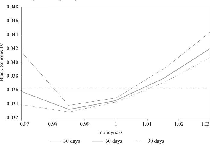
Figure 7 Implied volatility as a function of moneyness for the foreign currency European call option, ρ= – 0.461.
0.048
0.046
0.044
0.042
0.040
0.038
0.036
0.034
0.032
0.97 0.98 0.99 1 1.01 1.02 1.03
moneyness
60 days
30 days 90 days
Black-Scholes IV
a decreasing function of the maturity. For options near the money, (K/C = 1), if asym-metry is absent or very mild (ρ = 0 or ρ = -0.17074), the implied volatility is an increas-ing function of maturity. This is consistent with findincreas-ings of Shastri and Wethyavivorn (1987) and Duan (1999).
Figure 8 Implied volatility as a function of moneyness for the foreign currency European call option, ρ= 0.
0.043
0.042
0.041
0.040
0.039
0.038
0.037
0.036
0.035
0.034
0.97 0.98 0.99 1 1.01 1.02 1.03
moneyness
60 days
30 days 90 days
Black-Scholes IV
5 Conclusion
parameter estimation procedure using the time series of the underlying process X. But, once the data from the options market are at our disposal, it will be possible to conduct the analysis and the parameter estimation using data from options market only. In that case, it would be interesting to analyze whether the predictions for option prices obtained using the NGARCH model differ from those observed on the market. Also it would be interesting to measure to what extent it results in the improvement of the estimating pro-cedure for prediction purposes. Since in the non-linear asymmetric GARCH framework it is possible to model the correlation of the conditional variance and lag returns, the model can be especially useful even for modelling stocks, and thus options on stocks, because of the well known leverage effect phenomenon (e. g. Christie, 1982). This indicates the possibility of applying the NGARCH model for option pricing on every asset of interest on the Croatian stock exchange. Furthermore, once the data from the options market are accessible, it will be interesting to explore how the predicted option prices can be im-proved using models with jump processes since such models can explain unpredictable market movements. Finally, once the options market is founded, there will be a variety of models trying to model different phenomena.
Appendix 1
Proof for the local risk neutrality for the GARCH model
Let us suppose that process specifications under the new measure are given by (15) and (16). Supposing rational investor behaviour (in the sense that prefers more money to less), the foreign currency is a special case of the foreign asset given by the relation
Xt =Ctexp(r ts ). (25)
Since from the model assumptions σ2
t+1 is the value known at time t, and Z* is a standard normal random variable, from specification (15) it follows that ln(Xt+1/Xt) = rs + ln(Ct+1/Ct) is conditionally normal distributed random variable thus Xt+1/Xt is conditionally
log-normal.
Furthermore, calculating the conditional expectation of the relation (15) it follows that E Xt*[ t+1/Xt] = E Ct*[ t+1exp( (r ts +1)) / (Ctexp(rstt
r Es t rd rs t t Zt
))]
= ( ) [ ( 1
2 *
1 2
1 1
exp exp − − σ + +σ + **+
1
2 *
1 *1
)]
= ( 1
2 ) [ ( )].
exprd− σt+ Et expσt+Zt+ (26)
But, σ2
t+1Z*t+1 is conditionally normal distributed random variable of zero expectation and variance σ2
t+1, so the expression E*t [exp(σt+1Z*t+1)] represents the moment generating function for the normal random variable calculated in 1 which is exactly exp(1
2 1). 2 σt+ So,
E X*t[ t+1/Xt] =exp( )rd , (27)
which fulfils the second condition.
Finally, taking into consideration that the variance of tomorrow’s return, σ2
t+1, which is known at the end of today’s day, i. e. in time t, and using relations (15) and (16) it fol-lows that
Vart*[ (ln Xt+1/Xt)] = Et*[ω α σ+ ( tZt*−λσt −ρσt)2+ββσ
ω α σ λσ ρσ βσ
t
t t d s t t t t
E P r r
2
* 2 2
]
= [ ( 1
2 )
+ − + + − − + 22
2 2 1 ] = [ ( ) ] = [ ( / E Z
Var X X
t t t t t
t t t
ω α σ+ −ρσ +βσ
+
ln ))], (28)
where the last equality follows from relation (3). This fulfils the third condition. Appendix 2
Foreign currency option prices under the GARCH model and the Black-Scholes model for different maturities and strikes with volatility σ0 = 0.036128 currency spot price C = 7.335 and parameters from Table 122
Days to maturity τ m Strike coGH coBS
30 0.97 1.00 1.00 1.02 1.03 7.12 7.22 7.34 7.45 7.56 0.22308690122941 0.11741870260476 0.03721059194186 0.00624557117497 0.00080196491670 0.22288483536895 0.11766584897751 0.03812329096746 0.00563250518454 0.00030742586018 60 0.97 1.00 1.00 1.02 1.03 7.12 7.22 7.34 7.45 7.56 0.22756291771718 0.12794447130915 0.05362443201262 0.01624776243006 0.00392655032981 0.22720379640897 0.12867323461609 0.05477715335458 0.01581733927356 0.00287215360745 90 0.97 1.00 1.00 1.02 1.03 7.12 7.22 7.34 7.45 7.56 0.23210542851231 0.13733693276207 0.06638849391364 0.02594685840856 0.00857959351282 0.23267520409955 0.13898858113885 0.06784528392649 0.02563837476337 0.00720066693796
22In the table are presented results which have the estimated unconditional value σ2
0 as the initial value of the
Appendix 3
Foreign currency option prices under the GARCH and the Black-Scholes model for different maturities and strikes with volatility σ0 = 0.036128, currency spot price C = 7.335 and ρ = -0.461
Days to maturity τ m Strike coGH coBS
30 0.97 1.00 1.00 1.02 1.03 7.12 7.22 7.34 7.45 7.56 0.22329682837468 0.11663240889513 0.03681841852915 0.00738232725972 0.00140489838562 0.22288483525001 0.11766584778476 0.03812328834133 0.00563250382702 0.00030742568463 60 0.97 1.00 1.00 1.02 1.03 7.12 7.22 7.34 7.45 7.56 0.22711154073123 0.12581817310359 0.05224104494910 0.01770478546070 0.00587851654204 0.22720379566394 0.12867323219096 0.05477714965717 0.01581733654321 0.00287215259940 90 0.97 1.00 1.00 1.02 1.03 7.12 7.22 7.34 7.45 7.56 0.23137836550745 0.13472117261886 0.06468078932117 0.02735599257122 0.01151890310116 0.23267520260550 0.13898857779652 0.06784527941821 0.02563837101399 0.00720066497420 Appendix 4
Foreign currency option prices under the GARCH and the Black-Scholes model for different maturities and strikes with volatility σ0 = 0.036128, currency spot price C = 7.335 and ρ = 0.
Days to maturity τ m Strike coGH coBS
REFERENCES
Bernstein, P., 1992. Capital Ideas: The Improbable Origins of Modern Wall Street.
New York: Free Press.
Black, F. and Scholes, M., 1973. “The Pricing of Options and Corporate Liabilities”.
Journal of Political Economy, 81 (3), 637-654.
Bollerslev, T., 1986. “A generalized autoregressive conditional heteroscedasticity”.
Journal of Econometrics, 31, 307-327.
Bollerslev, T., Chou, R. and Kroner, K., 1992. “ARCH Modeling in Finance: A re-view of the Theory and Empirical Evidence”. Journal of Econometrics, 52 (1-2), 5-59.
Campbell, J. Y., Lo, A. W. and MacKinlay, A. C., 1997. The Econometrics of Financial Markets. Princeton; New Jersey: Princeton University Press.
Christie, A. A., 1982. “The Stochastic Behaviour of Common Stock Variances: Value, Leverage and Interest Rate Effects”. Journal of Financial Economics, 10, 407-432.
Christoffersen, P. F., 2003. Elements of Financial Risk Management. San Diego: Academic Press.
Cont, R. and da Fonseca, J., 2002. “Dynamics of Implied Volatility Surfaces”.
Quantitative Finance, 2 (1), 45-60.
Cooper, I. [et al.], 1986. Option Hedging. Mimeo. London: London Business School.
Ding, Z., Granger, C. W. J. and Engle, R. F., 1993. “A Long Memory Property of Stock Market Returns and a New Model”. Journal of Empirical Finance, 1 (1), 83-106. Duan, J.-C., 1995. “The GARCH Option Pricing Model”. Mathematical Finance, 5 (1), 13-32.
Duan, J.-C., 1997. “Augmented GARCH (p, q) Process and its Diffusion Limit”.
Journal of Econometrics, 79 (1), 97-127.
Duan, J.-C., 1999. “Pricing Foreign Currency and Cross-Currency Options Under GARCH”. The Journal of Derivatives, 7 (1), 51-63.
Engle, R. F. and Ng, V. K., 1993. “Measuring and testing the impact of news on volatility”. Journal of Finance, 48 (5), 1749-1778.
Engle, R. F., 1982. “Autoregressive conditional heteroscedasticity with estimates of the variance of United Kingdom inflation”. Econometrica, 50 (4), 987-1007.
Engle, R. F., 1995. ARCH: Selected Readings. Oxford: Oxford University Press. Fama, E., 1965. “The behavior of stock market prices”. Journal of Business, 38 (1), 34-105.
Geske, R.,1979. “The Valuation of Compound Options”. Journal of Financial Economics, 3, 125-144.
Hentschel, L., 1995. “All in the Family: Nesting Symmetric and Asymmetric GARCH Models”. Journal of Financial Economics, 39 (1), 71-104.
Hull, J. and White, A., 1987. “The Pricing of Options on Assets with Stochastic Volatilities”. Journal of Finance, 42 (2), 281-300.
Johnson, H. and Shanno, D., 1987. “Option Pricing When the Vaiance is Changing”.
Journal of Financial and Quantitative Analysis, 22, 143-151.
Mandelbrot, B., 1963. “The variation of certain speculative prices”. Journal of Business, 36 (4), 394-419.
Merton, R., 1973. “The Theory of Rational Option Pricing”. Bell Journal of Economics and Management Science, 4 (1), 141-183.
Merton, R., 1976. “Option Pricing When Underlying Stock Returns are Discontinuous”. Journal of Financial Economics, 4, 141-183.
Nelson, D., 1991. “Conditional Heteroscedasticity in Asset Returns: A New Approach”. Econometrica, 59 (2), 347-370.
Rebonato, R., 1999. Volatility and Correlation in the pricing of Equity, FX and Interest Rate Options. Chichester: Wiley.
Rubinstein, M., 1983. “Displaced Diffusion Option Pricing”. Journal of Finance, 38 (1), 213-217.
Rubinstein, M., 1985. “Nonparametric Tests of Alternative Option Pricing Models Using all Reported Trades and Quotes on the 30 Most Active CBOE Option Classes from August 23, 1976 through August 31, 1978”. Journal of Finance, 40 (2), 455-480.
Scott, L., 1987. “Option Pricing When the Variance Changes Randomly: Theory, Estimation and an Application”. Journal of Financial and Quantitative Analysis, 22 (4), 419-438.
Shastri, K. and Wethyavivorn, 1987. “The Valuation of Currency Options for Alternate Stochastic Processes”. Journal of Financial Research, 10, 283-293.
Shephard, N. 1996. “Statistical aspects of ARCH and stochastic volatility” in: Time Series Models in Econometrics, Finance and Other Fields. London: Chapman and Hall, 1-67.
Stein, E. and Stein, J., 1991. “Stock Price Distributions with Stochastic Volatility: An Analytic Approach”. Review of Fianncial Studies, 4 (4), 727-752.
Šestović, D. and Latković, M., 1998. “Modeliranje volatilnosti vrijednosnica na Zagrebačkoj burzi”. Ekonomski pregled, 49 (4-5), 292-303.
Taylor, S. J. and Xu, X., 1994. “The Magnitude of Implied Volatility Smiles: Theory and Empirical Evidence for Exchange Rates”. Review of Future Markets, 13, 355-380.
Taylor, S., 1986. ModellingFinancial Time Series. New York: Wiley.