Theory and Application of the Generalized Integral Representation Method (GIRM) in Advection Diffusion Problem

(1)

2014; 3(4): 137-149

Published online August 10, 2014 (http://www.sciencepublishinggroup.com/j/acm) doi: 10.11648/j.acm.20140304.15

ISSN: 2328-5605 (Print); ISSN: 2328-5613 (Online)

Theory and application of the generalized integral

representation method (GIRM) in advection diffusion

problem

H. Isshiki

IMA (Institute of Mathematical Analysia), Osaka, Japan

Email address:

[email protected]

To cite this article:

H. Isshiki. Theory and Application of the Generalized Integral Representation Method (GIRM) in Advection Diffusion Problem.Applied and Computational Mathematics. Vol. 3, No. 4, 2014, pp. 137-149. doi: 10.11648/j.acm.20140304.15

Abstract:

The integral representation is developed for linear initial and boundary value problems. The fundamental

solution is defined by the linear differential equation with constant coefficients and plays a key role in obtaining the integral representation. This becomes a very strong constraint in developing the theory to nonlinear problems. In the present paper, an innovative generalization of the integral representation or generalized integral representation is proposed. The numerical examples are given to verify the theory.

Keywords:

Advection Diffusion Problem, Reciprocity, Integral Representation, Fundamental Solution, Generalization

1. Introduction

Wu [1] and Uhlman [2] obtained integral representations for Navier-Stokes equation using the fundamental solution for Laplace operator and showed clearly how to apply the integral representation method to nonlinear problems. Wu verified his theory through a series of numerical calculations. Isshiki, Nagata and Imai [3] has applied Uhlman’s idea to a viscous flow around a circular cylinder successfully.

In the present paper, an innovative generalization of the integral representation or Generalized Integral Representation (GIR) is proposed. The idea is applied to the problem of advective diffusion. Ordinary, we define the fundamental solution first and then apply it to obtain the integral representation. On the other hand, in the generalized theory, the fundamental function is chosen first, and the differential equation satisfied by the fundamental solution is defined properly reflecting the fundamental solution and the boundary value problem [4]. For example, we can use the Gaussian function as the generalized fundamental solution. This approach can extend the applicability of the integral representation method.

We conduct numerical calculations of 1D and 2D problems and demonstrate the effectiveness of Generalized Integral Representation (GIRM). Stable and precise results are obtained in an admissible time.

2. Generalized Integral Representation

in Diffusion Problem

2.1. Generalized Reciprocity

The advection-diffusion equation is given by

(

( , ) ( , )

)

( ,) ) , ( ) ) , ( ( ) , (

t t C t

t C t t

t C

x x x

x x

u x

x x

x

σ

κ ∇ +

⋅ ∇ =

∇ ⋅ + ∂ ∂

, (1)

where x and t are the coordinates and time, C, u , κ and σ are the density of material, advection velocity, diffusion constant and source of material, respectively. For convenience, we rewrite Eq. (1):

   

+ ⋅ −∇ = ∇

⋅ + ∂ ∂

∇ − =

) , ( ) , ( )

, ( ) ) , ( ( ) , (

) , ( ) , ( ) , (

t t t

C t t

t C

t C t t

x x q x

x u x

x x

x q

x x

x

σ κ

, (2)

(2)

       + ⋅ −∇ = ∇ ⋅ + ∂ ∂ ∇ − = ) , ( ) , ( ) , ( ) ) , ( ( ) , ( ) , ( ) , ( ) , ( t t t C t t t C t C t t P P P P P P x x q x x u x x x x q x x x σ κ

, (3)

and        + ⋅ −∇ = ∇ ⋅ − ∂ ∂ ∇ − = ) , ( ) , ( ) , ( ) ) , ( ( ) , ( ) , ( ) , ( ) , ( t t t C t t t C t C t t Q Q Q Q Q Q x x q x x u x x x x q x x x σ κ

. (4)

Now, we have

∫∫∫

               − ⋅ ∇ + ∇ ⋅ + ∂ ∂ = V Q P P P P t C t t t C t t t C ) , ( ) , ( ) , ( ) , ( ) ) , ( ( ) , ( 0 x x x q x x u x x x σ x x x x x x q x x u x dV t C t t t C t t t C P Q Q Q Q                − ⋅ ∇ + ∇ ⋅ − ∂ ∂ − ( , ) ) , ( ) , ( ) , ( ) ) , ( ( ) , ( σ

∫∫∫

_       ∂ ∂ − ∂ ∂ = V P Q Q P t C t t C t C t t C ) , ( ) , ( ) , ( ) , ( x x x x

(

)

(

)

_      ∇ ⋅ − ∇ ⋅ + ) , ( ) , ( ) ) , ( ( ) , ( ) , ( ) ) , ( ( t C t C t t C t C t P Q Q P x x x u x x x u x x

(

)

(

)

[

∇x⋅qP(x,t) CQ(x,t)− ∇x⋅qQ(x,t) CP(x,t)

]

+

[

xt C xt xt C xt

]

}

dVx P Q Q P ) , ( ) , ( ) , ( ) , ( σ σ + − +

∫∫∫

          ∂ ∂ − ∂ ∂ = V P Q Q P t C t t C t C t t C ) , ( ) , ( ) , ( ) , ( x x x x

(

)

(

)

_      ⋅ ∇ − ⋅ ∇ + ) , ( ) , ( ) , ( ) , ( ) , ( ) , ( t C t C t t C t C t Q P Q P x x x u x x x u x x

(

)

(

)

[

∇x⋅qP(x,t)CQ(x,t) −∇x⋅qQ(x,t)CP(x,t)

]

+

[

x t C xt xt C x t

]

}

dVx

P Q Q P ) , ( ) , ( ) , ( ) , ( σ σ + −

+ . (5)

Rewriting Eq, (5), we obtain

∫∫∫

V∂ _∂

Q P dV t C t t C x x x ) , ( ) , (

∫∫∫

∫∫

⋅ − + V Q P S Q P dV t C t dS t C

t nx x x x x x

x

q ( , ) ( , ) σ ( , ) ( , )

∫∫

⋅ + S Q P PQ dS t C t C

t nx x x x

x

u( , ) ( , ) ( , ) 2 1_ε

(

)

∫∫∫

∇ ⋅ − V Q P PQ dV t C t C t x

x u(x, ) (x, ) (x, )

2 1_ε

∫∫∫

∂ _∂ = V P Q dV t C t t C x x x ) , ( ) , (

∫∫∫

∫∫

⋅ − + V P Q S P Q dV t C t dS t C

t nx x x x x x

x

q ( , ) ( , ) σ ( , ) ( , )

∫∫

⋅ + S P Q QP dS t C t C

t nx x x x

x

u( , ) ( , ) ( , ) 2 1_ε

(

)

∫∫∫

∇ ⋅ − V P Q QP dV t C t C t x

x u(x, ) (x, ) (x, )

2 1_ε

, (6)

where 1 = − = QP PQ ε

ε . (7)

Equation (6) expresses the dynamic reciprocity between P and Q.

2.2. Generalized Integral Representation or 1-Step Generalized Integral Representation (1-GIRM)

Let’s define two solutions q and ~q as

    + ⋅ −∇ = ∇ ⋅ + ∂ ∂ ∇ − = ) , ( ) , ( ) , ( ) ) , ( ( ) , ( ) , ( ) , ( ) , ( t t t C t t t C t C t t x x q x x u x x x x q x x x σ κ (8) and        + ⋅ −∇ = ∇ ⋅ − ∂ ∂ ∇ − = ) , , ( ~ ) , , ( ~ ) , , ( ~ ) ) , ( ( ) , , ( ~ ) , , ( ~ ) , ( ) , , ( ~ t t t C t t t C t C t t ξ x ξ x q ξ x x u ξ x ξ x x ξ x q x x x δ κ

, (9)

where δ~ is a given function. Applying Eq. (6), we obtain

∫∫∫

V∂ _∂_t C t dV

t C x ξ x x ) , , ( ~ ) , (

∫∫∫

∫∫

⋅ − + V

Sq x t nxC xξt dSx x t C(x,ξ,t)dVx ~ ) , ( ) , , ( ~ ) , ( σ

∫∫

⋅ +

Su xt nxC xt C(x,ξ,t)dSx ~ ) , ( ) , ( 2 1

(

)

∫∫∫

∇ ⋅ −

V x u x t C x t C(x,ξ,t)dVx ~ ) , ( ) , ( 2 1

∫∫∫

∂ _∂ =

V _t C t dV

t C x x ξ x ) , ( ) , , ( ~

∫∫∫

∫∫

⋅ − + V

Sq xξt nxC xt dSx (x,ξ,t)C(x,t)dVx ~ ) , ( ) , , ( ~ _δ

∫∫

⋅ −

(3)

(

)

∫∫∫

∇ ⋅

+

V x u xt C(x,ξ,t)C(x,t)dVx ~ ) , ( 2 1

. (10)

Rewriting

∫∫∫

V (x,ξ,t)C(x,t)dVx ~ δ

∫∫∫

+ ∂ _∂ ∂ ∂ − = V

V _t C t dV

t C dV t C t t C x x x ξ x ξ x x ) , ( ) , , ( ~ ) , , ( ~ ) , (

∫∫

⋅ + ⋅ − S

Sq x t nxC xξt dSx q(x,ξ,t) nxC(x,t)dSx ~ ) , , ( ~ ) , (

∫∫∫

+

V xt C(x,ξ,t)dVx ~ ) , ( σ

∫∫

⋅ −

Su x t nxC(x,ξ,t)C(x,t)dSx ~ ) , (

(

)

∫∫∫

∇ ⋅ +

V x u xt C(x,ξ,t)C(x,t)dVx ~

) ,

( _{. (11)}

Exchanging x and ξ, we obtain a generalized integral representation (GIR):

∫∫∫

_V (ξ,x,t)C(ξ,t)dVξ

~ δ

∫∫∫

+ ∂ _∂ ∂ ∂ − = V

V _t C t dV

t C dV t C t t C ξ ξ x x ξ x ξ ξ ) , ( ) , , ( ~ ) , , ( ~ ) , (

∫∫

⋅ + ⋅ − S

Sq ξt nξC ξxt dSξ q(ξ,x,t) nξC(ξ,t)dSξ ~ ) , , ( ~ ) , (

∫∫∫

+

V ξt C(ξ,x,t)dVξ ~ ) , ( σ

∫∫

⋅ −

Su ξt nξC(ξ,x,t)C(ξ,t)dSξ ~ ) , (

(

)

∫∫∫

∇ ⋅ +

V ξ u ξt C(ξ,x,t)C(ξ,t)dVξ ~

) ,

( _{. (12)}

If δ~(x,ξ,t) is Dirac’s delta function ) ( ) ( ) ( ) , , (

~ _δ _ξ _δ _η _δ _ζ

δ xξt = x− y− z− , the integral on the left-hand side of Equation (12) becomes C(x,t). However, when the convection velocity u(x,t) and the diffusion constant κ(x,t) are not a constant vector and number, respectively, the analytical solution of ~q(x,ξ,t) and

) , , ( ~ t

C xξ can’t be obtained. Instead, we can specify

) , , ( ~ t

C xξ first and determine δ~(x,ξ,t) next. For example, if we use the Gaussian function for C~(x,ξ,t):

        ₋ − = = 2 2 2 3 2 2 | | exp ) 2 ( 1 ) , ( ~ ) , , ( ~ γ πγ ξ x ξ x ξ

x t C

C , (13)

where γ is assumed constant, but it could be a function of

ξ. If we apply the theory to a numerical procedure using an

irregular mesh, we must consider as γ =γ(ξ). Then, we have

) , ( ~ ) , ( ) , , (

~ _x_ξ _x _x _ξ

q t =−κ t∇C

                ₋ − ∇ −

= ₂ ₃₂ ₂2

2 | | exp ) 2 ( 1 ) , ( γ πγ

κ xt x x ξ , (14a)

(

( , ) ~( , ,)

)

( ( , ) )~( , , ) ) , , ( ~ t C t t C t

t x xξ ux xξ

ξ

x =−∇x⋅κ ∇ − ⋅∇x

δ         ₋ − ∇ ⋅ −

= ₂ ₃₂ ₂ 2

2 | | exp ) 2 ( 1 ) ) , ( ( γ πγ ξ x x

u t _x

                ₋ − ∇ ⋅ ∇ − 2 2 2 3 2 2 | | exp ) 2 ( 1 ) , ( γ πγ

κ x x ξ

x t , (14b)

where ) ( ) ( ) ( |

| 3 3

2 2 2 2 1

1−ξ + −ξ + −ξ

= −

= x x x

r x ξ . (15)

Furthermore, when C~(x,ξ,t) is defined as Eq. (13), and γ tends to zero, then C~(x,ξ,t) and

δ

~

(

x

,

ξ

,

t

)

satisfy

) , ( ) , , ( ~ ξ x ξ

x t →δ

C , (16a)

[

( , ) ( , )

]

) , ( ) ) , ( ( ) , , ( ~ ξ x x ξ x x u ξ x x x x δ κ δ δ ∇ ⋅ ∇ − ∇ ⋅ − → t t t

, (16b)

where δ(x,ξ) is the Dirac’s delta function )

( ) ( )

( 1 ξ1 δ 2 ξ2 δ 3 ξ3

δ x − x − x − .

At an internal point (IP), the left-hand side of Eq. (12) becomes

(

( , ) ( , )

)

) , ( )) , ( ( ) , ( ) ) , ( ( t C t t C t t C t x x x x u x x u x x x x ∇ ⋅ ∇ − ⋅ ∇ + ∇ ⋅ →

κ , (17)

since

∫∫∫

V (ξ,x,t)C(ξ,t)dVξ ~ δ

(

)

∫∫∫

        ∇ ⋅ ∇ − ∇ ⋅ − →

V _t C t dV

t ξ ξ ξ ξ ξ x ξ ξ x ξ ξ u ) , ( ) , ( ) , ( ) , ( ) ) , ( ( δ κ δ ) , ( )) , ( ( ) , ( ) ) , (

(u xt ⋅∇x C xt + ∇x⋅u xt C xt =

[

]

∫∫∫

∇ ⋅∇

+

V κ(ξ,t) ξδ(ξ,x) ξC(ξ,t)dVξ

(

( , ) ( , )

)

) , ( )) , ( ( ) , ( ) ) , ( ( t C t t C t t C t x x x x u x x u x x x x ∇ ⋅ ∇ − ⋅ ∇ + ∇ ⋅ =

κ . (18)

(4)

(

( , )

)

( , ) ) , ( ) , ( t C t t t t C x x u x x x⋅ ∇ + + ∂ ∂ −

→ σ , (19)

since t t C dV t C t t C dV t C t t C V V ∂ ∂ − → ∂ ∂ + ∂ ∂ −

∫∫∫

) , ( ) , ( ) , , ( ~ ) , , ( ~ ) , ( x x x ξ x ξ ξ ξ ξ

, (20a)

0 ) , ( ) , , ( ~ ) , , ( ~ ) , ( → ⋅ + ⋅ −

∫∫

S S dS t C t dS t C t ξ ξ ξ ξ ξ n x ξ q x ξ n ξ q

, (20b)

) , ( ) , , ( ~ ) ,

( t C t dV t

Vσ ξ ξx ξ →σ x

+

_∫∫∫

, (20c)

0 ) , ( ) , , ( ~ ) , ( ⋅ → −

_∫∫

Suξ t nξC ξ xt C ξt dSξ , (20d)

(

)

(

( , )

)

( , ) ) , ( ) , , ( ~ ) , ( t C t dV t C t C t V x x u ξ x ξ ξ u x ξ ξ ⋅ ∇ → ⋅ ∇ +

_∫∫∫

, (20e)

Hence, the generalized integral representation, Eq. (12), tends to the differential equation, Eq. (1), at IP.

If C(x,t) at an interior point (IP) and C(x,t) or

n t

C ∂

∂ (x, ) at a boundary point (BP) are known from the boundary conditions, then GIR given by Eq. (12) is an integral equation with ∂C(x,t) ∂t the unknown variable at IP and ∂C(x,t) ∂n or C(x,t) the unknown variable at BP. We obtain C(x,t+dt) at IP from

t t C dt t C dt t

C(x, + )= (x, )+ ∂ (x, ) ∂ . Hence, if C(x,0) on IP is known from the initial condition, then we can solve the initial and boundary value problem using GIR given by Eq. (12).

If we use another definition of Eq. (9), for example, ) , ( ) , (

G~ xξ δ xξ

2

x =

∇ , then, Eq. (12) becomes the ordinary integral representation in case of linear problem.

Now, we assume that the diffusion coefficient κ(x,t) and the abduction velocity u(x,t) are given simply by

const t =κ=

κ(x, ) , (21a)

const U t)= = , (x

u . (21b)

Furthermore, if we assume Eq. (13), Eqs. (14) and (12) are given by               ₋ − ∇ − = ∇ − = 2 2 2 3 2 2 | | exp ) 2 ( 1 ) , ( ~ ) , ( ) , , ( ~ γ πγ κ κ ξ x ξ x x ξ x q x C t t

, (22a)

(

( , ) ~( , , )

)

( ( , ) )~( , , ) ) , , ( ~ t C t t C t

t x xξ u x xξ

ξ

x =−∇x⋅κ ∇ − ⋅∇x δ                 ₋ − ∂ ∂ −

= ₂ ₃₂ ₂ 2

2 | | exp ) 2 ( 1 γ πγ ξ x x U                 ₋ − ∇

− 2 ₂ ₃₂ ₂ 2

2 | | exp ) 2 ( 1 ) , ( γ πγ

κ xt x x ξ , (22b)

∫∫∫

V (ξ,x,t)C(ξ,t)dVξ

~ δ

∫∫∫

∂ _∂

− =

V _t C t dV

t C ξ x ξ ξ ) , , ( ~ ) , (

∫∫

⋅ + ⋅ − S

Sq ξt nξC ξxt dSξ q(ξ,x,t) nξC(ξ,t)dSξ

~ ) , , ( ~ ) , (

∫∫∫

+

V ξt C(ξ,x,t)dVξ

~ ) , ( σ

∫∫

−

SnC t C t dS U (ξ,x, ) (ξ, ) ξ

~

ξ , (23)

where ∇x⋅u(x,t)=0 is assumed.

2.3. Further Generalization of the Integral Representation or 2-Step Generalized Integral Representation (2-GIRM)

We call the integral representation derived in 4.2 as 1-step integral representation. We further generalize the theory and derive 2-step integral representation. Now, we rewrite Eq. (2) as Non-uniformity equation: ) , ( ) ,

(xt C xt

θ =∇x . (24a)

Constitutive equation: ) , ( ) , ( ) ,

(xt xtθ xt

q =−κ . (24b)

Equilibrium equation: ) , ( ) , ( ) , ( ) ) , ( ( ) , ( t t t C t t t C x x q x x u x x x σ + ⋅ −∇ = ∇ ⋅ + ∂ ∂

, (24c)

where a new variable θ(x,t) is introduced. The, we define a generalized fundamental solution (GFS):

) , ( ~ ) , ( ~ ξ x δ ξ x =

∇G (25)

As a GFS, we can use the Gaussian function defined by Eq. (13). Now, we consider to obtain GIRs corresponding to the differential equations (24a) and (24c).

From Eqs. (24a) and (25), we have

[

]

{

∫∫∫

−∇

=

V G( , ,t) ( ,t) C( ,t)

~

0 xξ θx x x

[

x xξ δ xξ

]

}

x

xt G dV

C( , )∇ ~( , )−~( , ) −

∫∫∫

=

VG(x,ξ,t)θ(x,t)dVx

~

[

]

∫∫∫

∇ + ∇

−

V G xξ xC xt C xt xG(x,ξ)dVx

(5)

∫∫∫

+

VC x t δ(x,ξ)dVx ~

) ,

( ₍₂₆₎

Rewriting Eq. (26), we obtain

∫∫∫

=−

V

VCxtδxξ dVx G(x,ξ)θ(x,t)dVx

~ )

, ( ~ ) , (

[

]

∫∫∫

∇ + ∇

+

VGxξ xCxt Cxt xG(x,ξ)dVx

~ ) , ( ) , ( ) , ( ~

. (27)

Transforming the second integral on the right-hand side of Eq. (27), we derive

∫∫∫

=−

V

VCxtδxξ dVx G(x,ξ)θ(x,t)dVx ~

) , ( ~ ) , (

∫∫

+

SG(x,ξ)C(x,t)nxdSx

~

. (28)

Exchanging x and ξ in Eq. (28), we obtain

∫∫∫

=−

V

VCξt δξx dVξ G(ξ,x)θ(ξ,t)dVξ

~ )

, ( ~ ) , (

∫∫

+

SG(ξ,x)C(ξ,t)nξdSξ

~

. (29)

Equation (29) is a GIR replacing the differential equation (24a).

From Eqs. (24c) and (25), we have

[

x

]

x

ξ x δ ξ x x

q

x x q

x x

u x ξ x

dV

G t

t t

t C t t

t C G

V

∫∫∫

      

      

− ∇ ⋅ +

  

 

  

 

− ⋅ ∇ +

∇ ⋅ + ∂ ∂

=

) , ( ~ ) , ( ~ ) , (

) , ( ) , (

) , ( ) ) , ( ( ) , ( ) , ( ~

0 _σ

∫∫∫

∂ _∂

=

V _t dV

t C

G x

x ξ

x, ) ( , ) (

~

[

]

∫∫∫

⋅∇ −

+

V G xξ uxt x C xt G(x,ξ) (x,t)dVx ~

) , ( ) ) , ( )( , ( ~

σ

[

]

∫∫∫

∇ ⋅ + ⋅∇

+

VG xξ x qxt qxt xG(x,ξ)dVx

~ ) , ( ) , ( ) , ( ~

∫∫∫

⋅

−

Vqxt δ(x,ξ)dVx ~ ) ,

( _{. (30)}

Rewriting Eq. (30), we obtain

∫∫∫

⋅ = ∂ _∂

V

V _t dV

t C G dV

t x x

x ξ x ξ

x δ x

q( , ) ~( , ) ~( , ) ( , )

∫∫∫

⋅∇

+

VG(x,ξ)(u(x,t) x)C(x,t)dVx ~

∫∫∫

−

VG(x,ξ) (x,t)dVx

~ _σ

[

]

∫∫∫ ∇ ⋅ + ⋅∇

+

VGxξ x qxt qxt xG(x,ξ)dVx

~ ) , ( ) , ( ) , ( ~

.(31)

Transforming the second and forth integrals on the right-hand side of Eq. (31), we derive

∫∫∫

⋅ = ∂ _∂

V

V _t dV

t C G dV

t x x

x ξ x ξ

x δ x

q( ,) ~( , ) ~( , ) ( ,)

(

)

∫∫∫

∇ ⋅

−

V xG(x,ξ) u(x,t)C(x,t)dVx

~

∫∫

⋅

+ _SG(x,ξ)C(x,t)u(x,t) nxdSx

~

∫∫

∫∫∫ + ⋅

−

S

VGxξ xt dVx G(x,ξ)q(x,t)nxdSx

~ ) , ( ) , (

~ _σ

(32)

Exchnging x and ξ in Eq. (32), we obtain

∫∫∫

⋅ = ∂ _∂

V

V _t dV

t C G dV

t ξ ξ

ξ x ξ x

ξ δ ξ

q(,) ~(, ) ~(, ) (,)

(

)

∫∫∫

∇ ⋅

−

V ξG(ξ,x) u(ξ,t)C(ξ,t)dVξ

~

∫∫

⋅

+

SG(ξ,x)C(ξ,t)u(ξ,t) nξdSξ

~

∫∫

∫∫∫

+ ⋅

− _VGξx ξt dVξ _SG(ξ,x)q(ξ,t)nξdSξ

~ ) , ( ) , (

~ _σ

. (33)

Equation (33) is a GIR replacing the differential equation (24c).

We can obtain the solution using the following steps: Solution: From Eq. (29), C(x,t)→θ(x,t); from Eq. (24b), θ(x,t)→q(x,t) ; from Eq. (33),

t t C t t

C(x, ),q(x, )→∂ (x, ) ∂ ; ∂C(x,t) ∂t→C(x,t+dt) ; repeat

3. Numerical Results by 2-Step

Generalized Integral Representation

(2-GIRM)

Since numerical examples using 1-GIRM are given in Ref. [4], we discuss only the applications of 2-GIRM. We consider initial value problem in infinite region. We assume the boundary values at infinity are zero. For simplicity, Eq. (21) is assumed. The time evolution is calculated explicitly. More specifically, we use Euler method. The material source

σ

is assumed zero. We use the Gaussian type fundamental solutions in Appendix A.

From Eqs. (29), (24b) and (33), we have

∫∫∫

=−

V

VC ξt δξ x dVξ G(ξ,x)θ(ξ,t)dVξ ~

) , ( ~ ) ,

( _{, (34)}

) , ( ) ,

(xt θx t

q =−κ , (35)

∫∫∫

⋅ = ∂ _∂

V

V _t dV

t C G

dV

t ξ ξ

ξ x ξ x

ξ δ ξ

q( , ) ~( , ) ~( , ) ( , )

∫∫∫

∂ _∂

−

V C t dV

G

U ξ ξ

x ξ

) , ( ) , ( ~

ξ , (36)

respectively.

3.1. 1D Problem

We approximate the infinite region by a finite one

L x L< <

(6)

M L

dx=2 , xi=−L+idx, i=0,1,⋯,M , (37a,b)

) , (

) (

ndt x C

C i

n

i = , ( , )

) (

ndt xi n

i

θ

= , () ( , )

ndt x q

q i

n

i = . (38a,b,c)

The discretization of Eqs. (34), (36) and (35) is given for 1

, , 1 ,

0 −

= N

i ⋯ by

∑∫

−

= −

− −

= −

− =−

1

0

) ( 2

2 1

0

) ( 2

2 ( , )

~ )

, (

~ N

j

n j dx

j x

dx j

x i

N

j

n j dx

j x

dx j

x δ ξ xi dξC G ξ x dξθ , (39)

) ( )

( n

i n i

q =−κθ , (40)

∑ ∫

= −

= +

− −

=

= +

− _

   

∂ ∂

= 1

0 2 2

) ( )

( 1

0 2

2 ( , )

~ )

, (

~ j N

j dx j x

dx j x

n

j i

n j N

j j

dx j x

dx j

x i _t

C d x G q

d

x ξ ξ ξ

ξ δ

∑ ∫

−

=

= +

− ∂

∂

− 1

0 2 2

) (

) , ( ~ N

j

j dx j x

dx j x

n j i _d _C

x G

U ξ

ξ ξ

, (41)

Rewriting, we have for i=0,1,⋯,N−1

∑

−

= −

= =−

1

0 ) ( 1

0 ) (

N

j n j ij N

j n j

ijC G

D θ , (42)

) ( )

( n

i n i

q =−κθ , (43)

∑

= −

=

= −

=

= −

     

∂ ∂

= 1

0 ) ( 1

0

) ( )

( 1

0

N j

j n j ij N

j

n

j ij n

j N j

j

ij U H C

t C G q

D , (44)

respectively, where the matrices D, G and H are given by

∫

₋+

= 2

2 ( , )

~ dx j x

dx j

x i

ij x d

D δ ξ ξ, (45a)

∫

₋+

= 2

2 ( , )

~ dx j x

dx j

x i

ij G x d

G ξ ξ_{, (45b)}

∫

₋+ ∂ _∂

= 2

2

) , ( ~ dx j x

dx j x

i

ij d

x G

H ξ

ξ

ξ _{. (45c)}

The matrix G is nonsingular. Hence, if the algebraic vector C(n) is known, we can obtain the algebraic vector

) n (

θ solving Eq. (42). Then, the algebraic vector q(n) is determined by Eq. (43). Now, the algebraic vector

(

)

(n)

t ∂

∂C is obtained solving Eq. (44), and the algebraic vector C(n+1) is obtained explicitly by

dt t

n n

n

) ( )

( ) 1

( _

    

∂ ∂ + =

+ C

C

C . (46)

If we use the implicit method, the solution would be much more stabilized. However, for simplicity, we adopt the

explicit solution or Euler solution for the numerical examples below.

The initial condition is given by

 

 ₋ _≤ _≤

=

otherwise 0

4 4

2 | when ) 4 3 ( 1 ) 0 ,

(x L L x L

C . (47)

or

 

 − ≤ ≤

=

otherwise 0

4 4

2 | when ) 4 3 ( 1

) 0

( L L x L

Ci i . (48)

The exact solution for this problem is known as

∫

₋∞_∞ − − −

= ξ

πκ

ξ κ

ξ

d e

t C t

x

C t

Ut x

4 2 ) (

2 ) 0 , ( )

,

( . (49)

The spurious oscillation or numerical oscillation is reduced using the additional calculation at every time step given by [6]

) , ( ) , ( )

,

( ₂

2

dt t x C dx

dt t x C d dt t x

C + +α + → + , (50)

where α is a parameter to reduce the spurious oscillation. More specifically, we have

(

( 1) ( 1) ( 1)

)

( 1)

2 ) 1 (

2

1 ₊ ₊ ₊ ₊

+ ₊ ₋ ₊ _→ n

i n

i n i n i n

i C C C C

dx

C α . (51)

A temporal value of (n+1) i

C calculated by Eq. (46) is corrected by Eq. (51) before advancing to the time step

1

+

n .

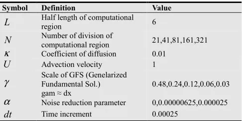
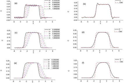
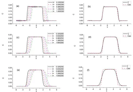
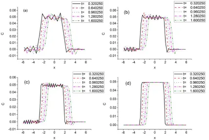
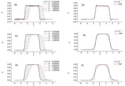
The parameters for the numerical calculations are shown in Tab. 1. The numerical results are shown in Figs. 1-3. As shown in Fig. 1, if the number of division N is increased, the computational errors are reduced, and the numerical solution converges to the exact one. Figures 2 and 3 show the effect of the noise reduction parameter α . The results are compared with those by the upwind differencing. The upwind differencing usually gives an excessive artificial or numerical diffusion. GIRM with noise reduction parameter

α gives more reasonable result.

Table 1. Parameters for numerical calculation.

Symbol Definition Value

L Half length of computational _region 6

N Number of division of _{computational region} 21,41,81,161,321

κ Coefficient of diffusion 0.01

U Advection velocity 1

γ Scale of GFS (Genelarized Fundamental Sol.) gam ≈ dx

0.48,0.24,0.12,0.06,0.03

α Noise reduction parameter 0,0.00000625,0.000025

(7)

Figure 1. Solution by GIRM (α =0; (a) N =21, γ =0.48; (b) N=41, γ =0.24; (c) N=81, γ =0.12; (d) N=161, γ =0.06; (e) N=321, γ =0.03; (f) exact solution)

Figure 2. Comparison among GIRM, FDM (upwind differencing) and exact solutions (N =41,γ =0.24; (a) GIRM, α =0; (b) GIRM, α =0,

6 . 1

=

t ; (c) GIRM, α=0.000025; (d) GIRM, α =0.000025, t=1.6; (e) FDM (upwind differencing); (f) FDM (upwind differencing),

6 . 1

=

(8)

Figure 3. Comparison among GIRM, FDM (upwind differencing) and exact solutions (N=81,γ =0.24; (a) GIRM, α=0; (b) GIRM, α =0,

6 . 1

=

t ; (c) GIRM, α =0.00000625; (d) GIRM, α =0.00000625, t=1.6; (e) FDM (upwind differencing); (f) FDM (upwind differencing),

6 . 1

=

t )

3.2. 2D problem

Before the discretization, we introduce a mapping of numbering from 2D numbering i=0,1,,⋯,M−1 ,

1 , , , 1 ,

0 −

= N

j ⋯ to 1D numbering iˆ=0,1,,⋯,MN−1:

i Mj

iˆ= + , (52a)

[ ]

i M i

i=ˆ− ˆ/ , j=

[ ]

iˆ/M . (52b)

We approximate the infini te region by a finite region

L x L< <

− , −B<y<B and discretize the finite region as

M L dx=2 ,

N B

dy= 2 , (53a)

dx i L

x_iˆ=− + , yiˆ=−B+ jdy. (53b)

The values at node

i

ˆ

are defined as )

ndt , ( C C(n) _iˆ

iˆ = x , ( iˆ,ndt) )

n ( i θ x

θ = , q_i(n)=q(x_iˆ,ndt) . (54a,b,c)

The discretization of Eqs. (34), (35) and (36) is given for 1

, , 1 ,

0 −

= M

i ⋯ by

∑∫

∫

∑ ∫

∫

− =

− −

+ − −

= − −

+ −

−

=

1

0

) (

ˆ 2

ˆ

2 ˆ

2

ˆ ˆ

1

0 ˆ

) ( ˆ 2

ˆ

2 ˆ

2

ˆ ˆ

)

,

(

~

)

,

(

~

N

j

n j dx

j x

dx j x

dy j y

dy j

y i

MN

j

n j dx

j x

dx j x

dy j y

dy j

y i

d

G

C

d

θ

x

ξ

x

ξ

δ

η

ξ

η

ξ

, (55)

) ( ˆ ) ( ˆ

n i n

i θ

q =−κ , (56)

) ( ˆ 1

0 ˆ

2 ˆ

2

ˆ ( , ˆ)

~ n

j MN

j dx j x

dx j x

dy j y

dy j

y δ ξxi d d ⋅q

∑ ∫

−

∫

= + −

+

− ξ η

∑ ∫

−

∫

= + −

+

− _

   

∂ ∂

= 1

0 ˆ

) (

ˆ 2

ˆ 2 ˆ

2 ˆ

2

ˆ ( , ˆ)

~ MN

j

n

j dx

j x

dx j x

dy j y

dy j

y i

t C d d Gξ x ξ η

) ( ˆ 1

0 ˆ

2 ˆ

ˆ)

, ( ~

n j MN

j dx j x

dx j x

dy j y

i _d _d _C

G

U

∑ ∫

∫

−

= + −

+

− _∂

∂

− ξ η

ξ

x ξ

, (57)

Rewriting, we have for iˆ=0,1,⋯,MN−1

∑

−

= −

=

−

= −

=

− =

1

0 ˆ

) (

ˆ ˆ ˆ 1

0 ) ( ˆ ˆ ˆ

1

0 ˆ

) (

ˆ ˆ ˆ 1

0 ˆ

) ( ˆ ˆ

MN

j n j y j i MN

j

n j j i y

MN

j n j x j i MN

j

n j j i x

G C

D

G C

D

θ θ

(9)

) (

ˆ )

( ˆ

n i x n

i x

q =−κθ , (ˆ) )

( ˆ

n i y n

i y

q =−κθ (59a,b)

∑

−

= −

=

−

= −

=

−

     

∂ ∂ =

+

1

0 ˆ

) ( ˆ ˆ ˆ 1

0 ˆ

) (

ˆ ˆ ˆ

) (

ˆ 1

0 ˆ ˆ )

( ˆ 1

0 ˆ ˆ

MN

j

n j j i MN

j

n

j j i

n j y MN

j j i y n

j x MN

j j i x

C H U t C G

q D q

D

, (60)

respectively, where the matrices (ρ=x,y), and are given by

∫

₋+

∫

₋+

= ˆ 2

2 2 2

ˆ ˆ

ˆ

ˆ ( , )

~ dx

j x

dx j x

dy j y

dy j

y i

j

i d d

D_ρ δ_ρ ξ x ξ η_{, (61a)}

∫

₋+

∫

₋+

= ˆ 2

2 ˆ

2

ˆ ˆ

ˆ

ˆ ( , )

~ dx

j x

dx j x

dy j y

dy j

y i

j

i G d d

G ξ x ξ η, (61b)

∫

₋+

∫

₋+ ∂ _∂

= ˆ 2

2 ˆ

ˆ ˆ

ˆ

) , ( ~ dx

j x

dx j x

dy j y

i j

i d d

G

H ξ η

ξ

x ξ

. (61c)

The matrix G is nonsingular. Hence, if the algebraic vector C(n) is known, we can obtain the algebraic vector

) n (

ρ

θ solving Eq. (55). Then, the algebraic vector q(_ρn) is determined by Eq. (56). Now, the algebraic vector

(

)

(n)

t

∂

∂C is obtained solving Eq. (57), and the algebraic vector (n+1)

C is obtained explicitly by

dt t

n n

n

) ( ) ( ) 1

( _

     ∂ ∂ + =

+ C

C

C . (62)

If we use the implicit method, the solution would be much more stabilized. However, for simplicity, we adopt the explicit solution or Euler solution for the numerical examples below.

The initial condition is given by

    

≤ ≤ −

≤ ≤ − =

otherwise 0

4 4

2 | and

4 4

2 when ) 16 9 ( 1 ) 0 , ,

( B y B

L x L BL

y x

C . (63)

or

    

≤ ≤ −

≤ ≤ − =

otherwise 0

4 4

2 | and

4 4

2 when ) 16 9 ( 1

ˆ ˆ )

0 (

ˆ B y B

L x L BL

C _i

i

i . (64)

The exact solution for this problem is known as

∫ ∫

₋∞_∞ ₋∞_∞ − − − + −

= ξ η

πκη

ξ ξ _κ η

d d e

t C t

y x

C t

y Ut x

4 2 ) ( 2 ) (

4 ) 0 , , ( )

, ,

( . (65)

The spurious oscillation or numerical oscillation is

reduced using the additional calculation at every time step given by [6]

) , , (

) , ( ) , ( )

, ,

( ₂

2 2

2

dt t y x C

y dt t x C x

dt t x C dt

t y x C

+ →

   

 

∂ + ∂ + ∂

+ ∂ +

+ α

. (66)

where α is a parameter to reduce the spurious oscillation. More specifically, we have

(

)

(

)

(ˆ 1)

) 1 ( ˆ ) 1 ( ) 1 ( ˆ 2

) 1 (

1 ˆ ) 1 ( ˆ ) 1 (

1 ˆ 2 ) 1 ( ˆ

2 1

+ +

− + +

+

+ − + + +

+ _→

   

 

   

 

+ − +

+ −

+ n

i n

M i n i n

M i

n i n i n i n

i C

C C C dy

C C C dx

C α . (67)

A temporal value of ( 1) ˆ

+ n i

C calculated by Eq. (62) is corrected by Eq. (67) before advancing to the time step

1 + n .

The parameters for the numerical calculations are shown in Tab. 1. The numerical results are shown in Figs. 4-7. As shown in Fig. 4, if the numbers of division M and

N

are increased, the computational errors are reduced, and the numerical solution converges to the exact one. Figures 5 and 6 show the effect of the noise reduction parameter

α

. The results are compared with those by the upwind differencing. The upwind differencing usually gives an excessive artificial or numerical diffusion. GIRM gives more reasonable artificial diffusion.

Table 2. Parameters for numerical calculations

Symbol Definition Value

L, B Half length and breadth of _{computational region} 6

M, N Number of division of _{computational region} 21,41,61

κ Coefficient of diffusion 0.01

U Advection velocity 1

γ Scale of GFS (Genelarized Fundamental Sol.) gam ≈ dx, dy

0.48,0.24,0.16

α Parameter for noise reduction 0,0.0000125,0.0000 25

(10)

Figure 4. Solution by GIRM (α =0, y=0; (a) N =21, γ =0.48; (b) N =41, γ =0.24; (c) N=61, γ =0.16; (d) Exact solution)

Figure 5. Comparison among GIRM, FDM (upwind differencing) and exact solutions (N =21,γ =0.48, y=0; (a) GIRM, α =0; (a) GIRM,

0

=

α , t=1.6; (c) GIRM, α =0.000025; (d) GIRM, α =0.000025, t=1.6; (e) FDM (upwind differencing); (f) FDM (upwind differencing),

6 . 1

=

(11)

Figure 6. Comparison among GIRM, FDM (upwind differencing) and exact solutions (N=41,γ=0.24, y=0; (a) GIRM, α =0; (a) GIRM, α=0,

6 . 1

=

t ; (c) GIRM, α=0.000025; (d) GIRM, α=0.000025, t=1.6; (e) FDM (upwind differencing); (f) FDM (upwind differencing), t=1.6)

Figure 7. Comparison among GIRM, FDM (upwind differencing) and exact solutions (N =61,γ =0.16, y=0; (a) GIRM, α =0; (a) GIRM,

0

=

(12)

4. Conclusions

In the present paper, an innovative generalization of the integral representation or Generalized Integral Representation (GIR) was proposed. The idea was applied to the problem of advective diffusion. Ordinary, we define the fundamental solution first and then apply it to obtain the integral representation. On the other hand, in the generalized theory, the fundamental function is chosen first, and the differential equation satisfied by the fundamental solution is defined properly reflecting the fundamental solution and the boundary value problem. For example, we could use the Gaussian function as the generalized fundamental solution. This approach could extend the applicability of the integral representation method.

We conducted numerical calculations of 1D and 2D problems and demonstrated the effectiveness of Generalized Integral Representation (GIRM). Stable and precise results were obtained in an admissible time.

Appendix A. Generalized Fundamental

Solutions

We can define various types of generalized fundamental solutions. However, we show only four types below. Although the 3D forms are shown, the 1D and 2D forms can be obtained easily.

A.1. Gaussian Type

The generalized fundamental solution of Gaussian type in 3D is given by

) , ( ~ ) , ( ~ ) , ( ~ ) , ( ~

1 1

1 xξ G yη G zζ

G

G xξ = , (A1a)

where

    

 

 ₋

−

= 2

2 1

2 ) ( exp 2

1 ) , ( ~

γξ γ

π

ξ x

x

G . (A1b)

We have

      

 ₋

=

∫

ξ _γξ

2 2

1 ) , ( ~

0 1

x erf dx x G x

, (A2a)

      

 ₋

=

∫

ξ ξ ξ ξ _γ

2 2 1 ) , ( ~

0 1

x erf d

x

G , (A2b)

    

 

 ₋ ₋

−

    

 

 ₊ ₋

=

∫

₋+

γ

γ ξ

ξ

2 2 2

1

2 2 2

1 ) , ( ~

2 2

x dx x erf

x dx x erf d

x G

j

j dx

j x

dx j x

. (A3)

From Eq. (24)

) , 2 (

~ ) , 2 (

~

) , ( ~ )

, (

~ 2

2 2

2

x dx x G x dx x G

d x G d

x

j j

dx j x

dx j x dx

j x

dx j x

− − +

=

∂ ∂ =

_∫

∫

₋+ ₋+ ξ

ξ ξ ξ

ξ δ

. (A4)

A.2. Cos-Hyperbolic Type

The generalized fundamental solution of cos-hyperbolic type in 3D is given by

) , ( ~ ) , ( ~ ) , ( ~ ) , ( ~

1 1

1 xξ G yη G zζ

G

Gxξ = , (A5a)

where

(

ξ γ

)

γ π ξ

) ( cosh | |

1 )

, ( ~

1

− =

x x

G . (A5b)

We have

(

)

(

ξ γ

)

γ γ π

γ ξ ξ

ξ δ

) ( cosh | |

) ( sinh )

, ( ~ ) , ( ~

2 1

1 ₋

− −

= ∂ ∂ =

x x x

x G

x , (A6)

(

)

∫

₋+ = ₋+ 2 ₋

2 2

2 1 _| _|_cosh₍ ₎

1 )

, (

~ x_j dx

dx j x dx

j x

dx j

x G ξ xdξ π γ ξ _x γ dξ

[

tan ( ) tan ( )

]

| |

2 1 ( 2)γ 1 ( 2)γ γ

π

γ xj x dx xj x dx

e

e −+ − − −

− ₋

= . (A7)

From Eq. (24)

) , 2 (

~ ) , 2 (

~

) , ( ~ )

, ( ~

1 1

2 2

1 2

2 1

x dx x G x dx x G

d x G d

x

j j

dx j x

dx j x dx

j x

dx j x

− − +

=

∂ ∂ =

_∫

∫

₋+ δ ξ ξ ₋+ _ξξ ξ

. (A8)

A.3. Lucy Type

The following is an approximation to Dirac’s delta function proposed by Lucy [7]:

    

> −

≤ −    



 ₋

−    



 ₋

+ =

σ σ σ

σ σ

π

| | 0

| | | | 1 | | 3 1 1 16 105 ) , ( ~

3

ξ x

ξ x ξ x ξ x ξ

x

G _{. (A9)}

A.4. Traditional Type

The following is the well known fundamental solution of Laplace operator :

| | 4

1 )

, ( ~

ξ x ξ

x

− − =

π

G _{, (A10)}

3

| |

) ( 4

1 ) , ( )

, ( ~

ξ x

ξ x ξ

x ξ

x

− − = −∇

=

∇ G G _π _{. (A11)}

) ( ) , ( ~

2

ξ x ξ x

x = −

(13)

References

[1] Wu J.C., Thompson J.F., “Numerical solutions of time-dependent incompressible Navier-Stokes equations using an integro-differential formulations”, Computers & Fluids, (1973), 1, pp. 197-215.

[2] S. J. Uhlman, “An integral equation formulation of the equations of motion of an incompressible fluid”, NUWC-NPT Technical Report 10,086, 15 July, (1992). [3] H. Isshik, S. Nagata, Y. Imai, “Solution of Viscous Flow

around a Circular Cylinder by a New Integral Representation Method (NIRM)”, AJET, 2, 2, (2014), pp. 60-82. file:///C:/Users/l/Downloads/983-5001-1-PB%20(1).pdf [4] H. Isshik, S. Nagata, Y. Imai, “Solution of a diffusion

problem in a non-homogeneous flow and diffusion field by the integral representation method (IRM)”, Applied

Mathematics and Computation, 3(1), (2014), pp. 15-26. http://article.sciencepublishinggroup.com/pdf/10.11648.j.ac m.20140301.13.pdf

[5] H. Isshiki, “Improvement of Stability and Accuracy of Time-Evolution Equation by Implicit Integration”, Asian Journal of Engineering and Technology (AJET), Vol. 2, No. 2 (2014), pp. 1339–160.

file:///C:/Users/l/Downloads/1205-5161-1-PB.pdf

[6] H. Isshiki, A method for Reduction of Spurious or Numerical Oscillations in Integration of Unsteady Boundary Value Problem, AJET, 2, 3, (2014), pp. 190-202.

file:///C:/Users/l/Downloads/1360-5725-2-PB%20(2).pdf [7] L. B. Lucy, “A numerical approach to the testing of the

fission hypothesis”, The Astronomical Journal, vol. 82, no. 12 (1977), pp. 1013-1024.