R E S E A R C H
Open Access
The error analysis of Crank-Nicolson-type
difference scheme for fractional subdiffusion
equation with spatially variable coefficient
Pu Zhang
1,2and Hai Pu
1,3**Correspondence: [email protected] 1State Key Laboratory for Geomechanics and Deep Underground Engineering, China University of Mining and Technology, Xuzhou, Jiangsu 221116, P.R. China
3School of Mechanics and Civil Engineering, China University of Mining and Technology, Xuzhou, Jiangsu 221116, P.R. China Full list of author information is available at the end of the article
Abstract
A Crank-Nicolson-type difference scheme is presented for the spatial variable coefficient subdiffusion equation with Riemann-Liouville fractional derivative. The truncation errors in temporal and spatial directions are analyzed rigorously. At each time level, it results in a linear system in which the coefficient matrix is tridiagonal and strictly diagonally dominant, so it can be solved by the Thomas algorithm. The unconditional stability and convergence of the scheme are proved in the discreteL2 norm by the energy method. The convergence order is min{2 –α2, 1 +
α
}in the temporal direction and two in the spatial one. Finally, numerical examples are presented to verify the efficiency of our method.MSC: 65M06; 65M12; 65M15
Keywords: fractional subdiffusion equation; variable coefficient; finite difference; stability; convergence
1 Introduction
In recent years, fractional differential equations have captured great attention of research in different domains. This facts reflect the ability of fractional calculation to describe many phenomena in different disciplines such as semiconductors, mechanics, signal processing, porous media, anomalous diffusion, and so on [–]. Employing fractional derivatives to describe the procedure of anomalous diffusion, we get the time fractional subdiffusion equation [, , ]:
∂u(x,t)
∂t =D
–α t
Kr
∂u(x,t)
∂x
+f(x,t), ()
whereDt–α( <α< ) denotes the Riemann-Liouville fractional derivative operator de-fined as
D–α t u(t) =
Γ(α)
d dt
t
u(s)
(t–s)–αds. ()
Some researchers considered the similar form with Caputo derivative:
C D
α tu(x,t) =
∂u(x,t)
whereCDα
t denotes Caputo’s derivative operator defined by
C D
α tu(t) =
Γ( –α)
t
du(s)
ds (t–s)
–αds, α∈(, ). ()
We have the following relation between the Caputo and Riemann-Liouville fractional derivatives.
Lety(t) be an (m– ) times continuously differentiable function in the interval [,T] with
y(m)(t) integrable in [,T]. For everyp, if ≤m– ≤p≤m, then the Riemann-Liouville fractional derivativeDpty(t) exists, and the following equality holds []:
Dp ty(t) =
m–
j=
y(j)()tj–p
Γ( +j–p)+ C D
p ty(t)
= m–
j=
y(j)()tj–p
Γ( +j–p)+
Γ(m–p)
t
y(m)(s)
(t–s)p–m+ds. ()
Much remarkable work has been done theoretically for diffusion and fractional prob-lems [–]. Marin and Marinescu [] studied the asymptotic partition of total energy for the solutions of the mixed initial boundary value problem within the context of the thermoelasticity of initially stressed bodies, and Hameedet al.[] derived and analyzed a mathematical model subject to low Reynolds number and long wavelength approxima-tions in order to study the peristaltic motion of fractional second-grade fluid in a vertical tube. In the regard of numerical work for time-fractional diffusion equations, Langlands and Henry [] obtained an implicit numerical method for the homogeneous problem and discussed the accuracy and stability of their scheme. Zhuanget al.[] integrated the linear and nonlinear subdiffusion equations about the time variabletand then approxi-mated the obtained equivalent equations numerically with the idea of numerical integrals. Yuste and Acedo [] developed an explicit scheme and gave a strict proof of the stability of the explicit scheme, and then Yuste [] analyzed the weighted average finite difference scheme by the von Neumann method.
equation with Riemann-Liouville fractional derivative, where the discreteHnorm con-vergence was proved rigorously, and the maximum norm error estimate was given. Based on a Crank-Nicolson-type discretization, Wang and Vong [] proposed a second-order accuracy formula to approximate the time-fractional derivative and established a compact finite difference scheme for solving the modified anomalous fractional subdiffusion equa-tion. For more applications of the Crank-Nicolson scheme, we refer the reader to [–]. The works we listed are mostly focused on the subdiffusion equation with constant coef-ficient. However, many practical applications involved variable diffusion coefficients [– ]. For example, the flow of heat in a rod is constituted by composite heat-conducting ma-terials, which means that the diffusion coefficient may vary with space variable. In view of some external heat source, Zhao [] considered the Caputo-fractional subdiffusion equation with spatially variable coefficient:
C D
α tu(x,t) =
∂ ∂x
ϕ(x)∂u
∂x
+g(x,t). ()
Employing anL formula, she obtained the convergence of order –α in the temporal direction and fourth-order approximation order in space. Vonget al.[] considered the same equation under Neumann boundary conditions and obtained the global convergence of orderO(τ–α+h). Metzleret al.[] suggested the following fractional model equation for anomalous diffusion:
Ddw t P(r,t) =
rds–
∂ ∂r
rds–∂P(r,t)
∂r
, r> ,t> , ()
whereP(r,t) is the probability density of random walks on fractals,dw> is the anoma-lous diffusion exponent,dsis just the spectral dimension of the fractal, andds=
df dw withdf denoting fractal dimension of the underlying object. Employing () and neglecting the co-efficient
rds– (which has no impact on difference approximation), () can be transformed
into equation ().
Ifu(x,t) is suitably smooth in time, then we have the following relationship [, ]:
D–α t
C
Dαtu(x,t) =
∂u(x,t)
∂t . ()
Therefore, implementing the operatorD–α
t on both sides of (), we derive the following Riemann-Liouville fractional subdiffusion equation with spatially variable coefficient:
∂u(x,t)
∂t =D
–α t
∂ ∂x
ϕ(x)∂u
∂x
+f(x,t), ()
wheref(x,t) =D–α t g(x,t).
The content of this paper is organized as follows. In Section , we introduce essential no-tation and some preliminary lemmas and then construct the Crank-Nicolson-type finite difference scheme. The unique solvability, unconditional stability, and theL-norm con-vergence are proved in Section by the energy method. Some examples are listed in Sec-tion to verify our theoretical analysis and testify the validaSec-tion of our difference scheme. Finally, a brief conclusion ends this work.
2 Derivation of a CN-type difference scheme
Consider the following subdiffusion equation with spatially variable coefficient combined with initial boundary value conditions:
∂u(x,t)
∂t =D
–α t
∂ ∂x
ϕ(x)∂u
∂x
+f(x,t), <x<L, <t≤T, ()
u(,t) =Φ(t), u(L,t) =Φ(t), <t≤T, ()
u(x, ) =Ψ(x), ≤x≤L, ()
where <α< , and we suppose thatc≤ϕ(x)≤candϕ(x),f(x,t),Φ(t),Φ(t),Ψ(x) are sufficiently smooth functions.
For a finite difference approximation, we suppose thatMandNare two positive integers and let h=ML andτ =NT be space and temporal step lengths, respectively. Definexi=
ih, ≤i≤M,tn=nτ, ≤n≤N,Ωh={xi|≤i≤M},Ωτ ={tn|≤n≤N}, and, in addition,tk–
= (k–
)τ,xi– = (i–)h.
For any grid functionu={uni |≤i≤M, ≤n≤N}, we denote
δxuni–
=
h
uni –uni–, δxuni =
h
δxuni+
–δxuni–
, ()
un–
i =
uni +uni–, δtu n– i =
τ
uni –uni–. ()
The following lemmas are needed for our error analysis.
Lemma ([]) For <α< and y∈C[,tn],we have:
Γ(α)
t
y(s)ds
(tn–s)α – τ
α–
Γ( +α)
y(tn) – n–
k=
(an–k––an–k)y(tk) –an–y()
= n
k=
tk
tk–
Lτ,α,n(s)y(s)ds=O
τ+α, ()
where ak= (k+ )α–kα,and for s∈(tk–,tk),
Lτ,α,n(s) =
Γ( +α)
(tn–s)α–
s–tk–
τ (tn–tk)
α +tk–s
τ (tn–tk–)
α
. ()
Furthermore,
n
k=
tk
tk–
Lτ,α,n(s)ds≤
Γ( +α)
α
+ +α +α –
Lemma ([]) Let y∈C[t
k–,tk].Then
y(tk) +y(tk–) =
τ
y(tk) –y(tk–)
+τ y()
tk– +
sτ
+y()
tk– –
sτ
–sds. ()
Now we define the grid functionUin=u(xi,tn), ≤i≤M, ≤n≤N, and, in addition, denoteϕ(xi+
) byϕi+. Lemma Suppose u∈C[x
i,xi+].Then
δxUi+ =u
(x i+) +
h u
xi+ + h t –u
xi+ –
h
t
( –t)dt, ()
δxUi+ =u(xi+) +
h u()
xi+ +
h
t
+u()
xi+ –
h
t
( –t)dt, ()
δxUi+ =u(xi+) +
h u()
xi+ +
h
t
–u()
xi+ –
h
t
( –t)dt
+h
u ()(x
i+). ()
Proof Employing the Taylor expansion with integral remainder, we have:
Ui+=u(xi+) +
h
u (x
i+) +
h u
xi+ +
th
( –t)dt, ()
Ui=u(xi+) –
h
u (x
i+) +
h u
xi+ –
th
( –t)dt. ()
Then subtracting these two equalities, we get the first statement. The proofs of the other two are similar by using an expansion of higher order.
Now we analyze the truncation error of theLanalog for the Riemann-Liouville frac-tional derivative.
Lemma Let u(x,t)∈C,([,L]×[,T]),ϕ(x)∈C[,L].Then for the truncation error,
we have:
D–α t ∂ ∂x
ϕ(x)∂u
∂x
(xi,tn)
= τ α–
Γ( +α)
δx(ϕδxU)ni – n–
k=
(an–k––an–k)δx(ϕδxU)ki –an–δx(ϕδxU)i
+ t α– n
Γ(α)δx(ϕδxU)
where(R)ni = (R)ni + (R)ni,and
(R)ni≤ max≤x≤L
≤t≤T
D–α
t
∂ ∂x
ϕ∂u ∂x
+D–αt ∂
∂x
ϕ∂
u
∂x
+
ϕ(x)Dt–α∂ u
∂x
h, ()
(R)ni≤
Γ( +α)
α
+ +α +α–
+ α–
· max
≤x≤L ≤t≤T
∂
∂x∂t
ϕ(x)∂u
∂x
+
ϕ(x) ∂
u
∂x∂t
τ+α. ()
Proof LetD–α
t u=wandWin=w(xi,tn). Then
D–α t ∂ ∂x
ϕ(x)∂u
∂x
= ∂
∂x
ϕ(x)∂w
∂x
. ()
It follows from Lemma that
δx(ϕδxW)ni =
h
ϕi+ δxW
n
i+ –ϕi–δxW
n i–
=
h
ϕi+ w
x(xi+,tn) –ϕi–wx(xi–,tn)
+ h h
ϕi+ w
()
x (xi+,tn) –ϕi–w
()
x (xi–,tn)
+ϕi+ h
w()x
xi+ +
t
h
–w()x
xi+ –
t
h
( –t)dt
–ϕi– h
w()x
xi– +
t
h
–w()x
xi– –
t
h
( –t)dt
= ∂
∂x
ϕ(x)∂w
∂x
(xi,tn) + h
ϕw()x x(ξ,tn)
+h
ϕwx()x
xi+
t
h,tn
+ϕwx()x
xi–
t
h,tn
( –t)dt
+ϕi+ h
w()x
xi+ +
t
h,tn
–w()x
xi+ –
t
h,tn
( –t)dt
–ϕi– h
w()x
xi– +
t
h,tn
–w()x
xi– –
t
h,tn
·( –t)dt, ()
whereξ∈[xi–,xi+]. So we have
∂ ∂x
ϕ(x)∂w
∂x
where
(R)ni≤ max≤x≤L
≤t≤T
D–α
t
∂ ∂x
ϕ∂u ∂x
+D–αt ∂
∂x
ϕ∂
u
∂x
+
ϕ(x)Dt–α∂ u
∂x
h. ()
It follows from () and () that
δx(ϕδxW)ni =
D–α
t δx(ϕδxU)(xi,tn) = τ
α–
Γ( +α)
δx(ϕδxU)ni – n–
k=
(an–k––an–k)δx(ϕδxU)ki –an–δx(ϕδxU)i
+ t α– n
Γ(α)δx(ϕδxU) i + n k= tk
tk– Lτ,α,n(s)
∂
∂tδx(ϕδxu)(xi,s)ds. () Using similar analysis and applying Lemma again, we get
δx(ϕδxU)ni = ∂ ∂x
ϕ(x)∂u
∂x
xi+
t
h,tn
+ ∂
∂x
ϕ(x)∂u
∂x
xi–
t
h,tn
dt
+ ϕi+
∂u
∂x
xi+ +
t
h,tn
–∂ u
∂x
xi+ –
t
h,tn
( –t)dt
– ϕi–
∂u
∂x
xi– +
t
h,tn
–∂ u
∂x
xi– –
t
h,tn
( –t)dt. ()
Applying () and the last equality, it is not hard to get
(R)ni≤
Γ( +α)
α
+ +α +α–
+ α–
· max
≤x≤L ≤t≤T
∂x∂∂t
ϕ(x)∂u
∂x
+
ϕ(x) ∂
u
∂x∂t
τ+α. ()
The proof is completed.
We now construct a Crank-Nicolson-type scheme for problem ()-(). Considering equality () at the point (xi,tn), we have
∂u(xi,tn)
∂t =D
–α t ∂ ∂x
ϕ(x)∂u
∂x
(xi,tn) +f(xi,tn), <n<N, <i<M– . ()
Then
∂u(xi,tn)
∂t +
∂u(xi,tn–)
∂t = D–α t ∂ ∂x
ϕ(x)∂u
∂x
(xi,tn) +Dt–α
∂ ∂x
ϕ(x)∂u
∂x
(xi,tn–)
+
From Lemma we obtain
∂u(xi,tn)
∂t +
∂u(xi,tn–)
∂t
=δtU n–
i + (R)ni, ()
where
(R)ni =
τ
∂u
∂t
xi,tn– + sτ +∂ u
∂t
xi,tn– –
sτ
–sds. ()
It follows from Lemma that
D–α t ∂ ∂x
ϕ(x)∂u
∂x
(xi,tn) +D–αt
∂ ∂x
ϕ(x)∂u
∂x
(xi,tn–)
=t α– n +tnα––
Γ(α) δx(ϕδxU) i
+ τ
α–
Γ( +α)
δx(ϕδxU)ni – n–
k=
(an–k––an–k)δx(ϕδxU)ki –an–δx(ϕδxU)i
+ τ
α–
Γ( +α)
δx(ϕδxU)ni–– n–
k=
(an–k––an–k–)δx(ϕδxU)ki –an–δx(ϕδxU)i
+ (R)
n i +
(R)
n–
i . ()
DenotingUn–
i =(Uin+Uin–) andδx(ϕδxU) n–
i =[δx(ϕδxU)in+δx(ϕδxU)ni–] and notic-ing that
– n–
k=
(an–k––an–k–)δx(ϕδxU)ki–an–δx(ϕδxU)i
= – n–
l=
(an–l––an–l)δx(ϕδxU)li––an–δx(ϕδxU)i
= – n–
l=
(an–l––an–l)δx(ϕδxU)li–+ (an––an–)δx(ϕδxU)i –an–δx(ϕδxU)i
= – n–
k=
(an–k––an–k)δx(ϕδxU)ki––an–δx(ϕδxU)i, ()
we have D–α t ∂ ∂x
ϕ(x)∂u
∂x
(xi,tn) +Dt–α
∂ ∂x
ϕ(x)∂u
∂x
(xi,tn–)
=t α– n +tnα––
Γ(α) δx(ϕδxU) i +
(R)
n i +
(R)
n– i +
τα–
Γ( +α) ·
δx(ϕδxU)ni – n–
k=
(an–k––an–k)δx(ϕδxU)ki –an–δx(ϕδxU)i
+ τ α–
·
δx(ϕδxU)ni–– n–
k=
(an–k––an–k)δx(ϕδxU)ki––an–δx(ϕδxU)i
=t α– n +tnα––
Γ(α) δx(ϕδxU) i + (R)
n– i +
τα–
Γ( +α) ·
δx(ϕδxU) n– i –
n–
k=
(an–k––an–k)δx(ϕδxU) k–
i –an–δx(ϕδxU)i
. ()
Substituting () and () into (), we have
δtU n– i =
τα–
Γ( +α)
δx(ϕδxU) n– i –
n–
k=
(an–k––an–k)δx(ϕδxU) k– i
–an–δx(ϕδxU)i
+t α– n +tα–n–
Γ(α) δx(ϕδxU) i +f
n–
i + (R)ni, ()
where (R)n i = (R)
n–
i – (R)ni, ≤i≤M– , ≤n≤N.
Whenn= , using equality () at the point (xi,t) and employing the Taylor expansion, we have
δtU
i =
∂u
∂t(xi,t) – (R)i
=Dt–α ∂
∂x
ϕ(x)∂u
∂x
(xi,t) +f(xi,t) – (R)i, ()
where
(R)i=τ
∂u
∂t(xi,sτ)s ds. () Using Lemma , we arrive at
δtU
i =
τα– Γ( +α)
δx(ϕδxU)i–aδx(ϕδxU)i +
τα–
Γ(α)δx(ϕδxU) i
+f(xi,t) + (R)i– (R)i
= τ α–
Γ( +α)
δx(ϕδxU)i+ (α– )δx(ϕδxU)i +fi+Ri, ()
where
Ri= (R)i– (R)i, ≤i≤M– .
By the previous analysis there exists a constantC, independent ofhandτ, satisfying
Rni≤Cτ+α+h, ≤i≤M– , ≤n≤N, () |Ri| ≤C
The initial and boundary conditions can be written as
Un=Φ(tn), UMn =Φ(tn), ≤n≤N, ()
Ui=Ψ(xi), ≤i≤M. ()
Ignoring the truncation errorsRni in () andRiin () and replacing the grid functionUin with its numerical analoguni, we arrive at the following difference scheme:
δtu n– i =
τα–
Γ( +α)
δx(ϕδxu) n– i –
n–
k=
(an–k––an–k)δx(ϕδxu) k–
i –an–δx(ϕδxu)i
+t α– n +tα–n–
Γ(α) δx(ϕδxu) i +f
n–
i , ≤i≤M– , ≤n≤N, ()
δtu
i =
τα– Γ( +α)
δx(ϕδxu)i+ (α– )δx(ϕδxu)i +fi, ≤i≤M– , ()
un=Φ(tn), unM=Φ(tn), ≤n≤N, ()
ui =Ψ(xi), ≤j≤M. ()
It is easy to see that, at each time level, the difference scheme ()-() is a tridiagonal system with strictly diagonal dominant coefficient matrix, and thus the difference scheme has a unique solution, and the Thomas algorithm suits.
3 Analysis of stability and convergence of the CN-type difference scheme 3.1 Stability
Now we introduce necessary notation and lemmas, which will be used in the analysis of stability and convergence.
Define the grid function spaceSh={u|u= (u,u, . . . ,uM),u=uM= }onΩh. For any
v,w∈Sh, we define the discrete inner products and corresponding norms as follows:
(v,w)h=h
M–
i=
viwi, v=
(v,v)h,
v,w=h
M–
i= (δxvi+
)(δxwi+), δxv=
v,v,
(δxu,δxv)ϕ=h M–
i=
ϕ(xi+
)(δxui+)(δxvi+), δxuϕ=
(δxu,δxu)ϕ, v∞= max
≤i≤M|vi|.
Considering the smoothness ofϕ(x), it is not hard to get √
cδxu ≤ δxuϕ≤ √
cδxu. ()
Lemma ([]) For any grid function u∈Sh,
u ≤√L
We have the following properties ofan.
Lemma
=a>a>a· · ·>an→, ()
α(n+ )α–<an<αnα–, ()
an–<
αnα–+α(n– )α– , n≥, () ˆ
an–<an–, aˆn–<an––an–, n≥, ()
whereaˆn–=[αnα–+α(n– )α–] –an–.
Proof Noticing thatan=α
n+
n xα–dxandxα–is a strictly convex and decreasing func-tion, the first three relations hold.
From inequalities ()-() we have
an––
αnα–+α(n– )α– > αnα––α(n– )α– () =αnα–
–
n n–
–α
> ()
and
an–>α(n– )α–>
αnα–+α(n– )α– , ()
so that () holds.
We now give the proof of the stability of the difference scheme ()-() with respect to the initial valueu
i and the inhomogeneous termf. We denote
f=,f,f, . . . ,fM–,
and
fn– =,fn–
,f n– , . . . ,f
n– M–,
, ≤n≤N.
Theorem Let umi , ≤i≤M, ≤m≤N,be a solution of the finite difference scheme
()-()withΨ=Ψ= .Then we have
um≤u+ τ α
Γ( +α)
( –α)+ δxuϕ
+ L
c
Γ( +α)τ–α·f
+ L
c·
Γ(α)τ·T–α
m
n=
Proof Taking the inner product of () withun–, we have
δtun–
,un–= τ
α–
Γ( +α)
δx(ϕδxu)n–
,un––
n–
k=
(an–k––an–k)
·δx(ϕδxu)k–
,un–+aˆ
n–
δx(ϕδxu),un–
+fn–,un–. ()
Noticing that
δtun–
,un–=
τu
n
–un–
and using the discrete Green formula and zero boundary conditions for every term in the right-hand side, we obtain
un–un–
τ =
τα–
Γ( +α)
–δxun–
,δ
xun–
ϕ+ n–
k=
(an–k––an–k)
·δxuk–
,δxun–
ϕ–aˆn–
δxu,δxun–
ϕ
+fn–,un–. ()
Applying the Cauchy-Schwarz inequality, we have
un–un–
τ ≤
τα–
Γ( +α)
–δxun–
ϕ+
n–
k=
(an–k––an–k)
·δxuk–
ϕ+δxu n–
ϕ
+aˆn– δxu
n– ϕ+δxu
ϕ
+fn–,un–. ()
Letting Γτ(+r–r)=I, we have
un–un–
Iτ ≤–δxu
n–
ϕ+ (a–an–)δxu n–
ϕ+
I|
fn–,un–|
+ n–
k=
(an–k––an–k)δxuk–
ϕ+aˆn–δxu n–
ϕ+δxu
ϕ
= (aˆn––an–– )δxun–
ϕ
+aˆn–δxuϕ+ n–
k=
(an–k––an–k)δxuk–
ϕ
+
If
From () we know that
un–un–
Iτ ≤ –δxu
n–
ϕ+ (an––an–)δxu ϕ + n– k=
(an–k––an–k)δxuk–
ϕ+
If
n–,un–.
Summing up for ≤n≤mand changing the summation order in the third term of the right-hand side, we get
um–u
Iτ ≤–
m
n=
δxun–
ϕ+ (a–am–)δxu ϕ + m– k= m
n=k+
(an–k––an–k)δxuk–
ϕ+ I m n=
fn–,un–
= – m
k=
δxuk–
ϕ+ m– k=
(a–am–k)δxuk–
ϕ
+ (a–am–)δxu ϕ+ I m n=
fn–,un–
= m–
k=
(–am–k)δxuk–
ϕ–δxu m–
ϕ+ I m n=
fn–,un–
+ (a–am–)δxu
ϕ+δxu ϕ = m k=
(–am–k)δxuk–
ϕ+ (a–am–)δxu
ϕ+δxu ϕ + I m n=
fn–,un–. ()
Using the Cauchy inequality, (), and Lemma , we have
If
n–,un–≤ L cIam–n
fn–+a
m–nδxun–
ϕ. ()
Substituting () into (), we have
um≤u+Iτ(a–am–)δxu
ϕ+δxu ϕ + m n=
τL cIam–n
fn–. ()
Taking the inner product of () withun–, we have
u–u τ =I
–δxu,δxu
ϕ+ ( –α)
δxu,δxu
ϕ +
f,u
=I–δxu
ϕ+ ( –α)
δxu,δxu
ϕ +
so that
u=u+Iτ–δxu
ϕ+ ( –α)
δxu,δxu
ϕ + τ
f,u. ()
Substituting () into () and using the Cauchy-Schwarz inequality again, we arrive at
um≤u+Iτ–δxu
ϕ+ ( –α)
δxu,δxu
ϕ
+Iτaδxu ϕ+
m
n=
τL cIam–n
fn–+ τf,u
≤u– Iτδxu
ϕ+Iτ
( –α)+ δxuϕ
+ m
n=
τL
cIam–n
fn–+ Iτδxu
ϕ+
Lτ
Ic
f. ()
Noticing thatam–n>am–>αmα–>αNα–, we have m
n=
τL cIam–n
fn–≤ τL
cIαNα– m
n=
fn–
= L
c·
τ–αΓ( +α)
αNα– m
n=
fn–
= L
c·
Γ(α)τ·T–α
m
n=
fn–. ()
Then, substituting () into (), we get () for ≤m≤N, and () form= is obvious.
So the proof is completed.
3.2 Convergence
We now consider the convergence of the difference scheme ()-(). Let
eni =Uin–uni, ≤i≤M, ≤n≤N.
Subtracting ()-() from ()-() and ()-(), we get the equations for the error:
δte n– i =
τα–
Γ( +α)
δx(ϕδxe) n– i –
n–
k=
(an–k––an–k)δx(ϕδxe) k– i
+Rni,
≤i≤M– , ≤n≤N, ()
δte
i =
τα–
Γ( +α)δx(ϕδxe)
i+Ri, ≤i≤M– , ()
en= , enM= , ≤n≤N, ()
Then from Theorem we have
en≤ L
c
Γ( +α)τ–α· R+ L
c
τ Γ(α)T–α·
n
k=
Rk. ()
From () and () we have
en≤ L
c
Γ( +α)τ–αcτ+h + L
c
Nτ Γ(α)T–αcτ+α+h () ≤ L
c
Γ( +α)cτ–α +h + L
c
Γ(α)T–αcτ+α+h . ()
Letting
β=min
–α , +α
, cˆ=Lc
Γ(α) c
Lα+ T–α,
we have the convergence in theLnorm.
Theorem Suppose that problem()-()has a smooth solution u(x,t)in the domain
[,L]×[,T]and un
i, ≤i≤M, ≤n≤N,is a solution of the difference scheme()-().
Then
max
≤n≤N
uxi,tn
–uni≤ ˆcτβ+h. ()
Remark The Crank-Nicolson-type scheme involves two time levels for a Riemann-Liouville fractional subdiffusion equation with spatially variable coefficient. Therefore, we actually used recursion method to handle the analysis of stability. Then we get the convergence, and the convergence order in spatial direction is just two. It is difficult to improve the space accuracy by introducing a compact technique.
4 Numerical examples
In this section, we give two examples to testify the efficiency and convergence orders of our difference scheme.
Example Consider the following problem with zero initial value:
∂u(x,t)
∂t =D
–α t
∂ ∂x
x+ ∂u
∂x
+ex( +α)t+α
–ex(x+ )· Γ( +α)
Γ( + α), <x< , <t≤, ()
u(,t) =t+α, u(,t) =et+α, <t≤, ()
u(x, ) = , ≤x≤. ()
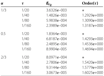
Table 1 The maximumL2errors and convergence orders for Example 1 whereh= 1/1,000
α τ EL2 Order(τ)
1/3 1/20 3.6326e–003 ∗
1/40 1.4826e–003 1.2929e+000 1/80 5.9838e–004 1.3090e+000 1/160 2.3989e–004 1.3187e+000
0.5 1/20 1.8364e–003 ∗
1/40 6.8187e–004 1.4293e+000 1/80 2.4895e–004 1.4536e+000 1/160 8.9904e–005 1.4694e+000
2/3 1/20 8.0971e–004 ∗
1/40 2.7806e–004 1.5420e+000 1/80 9.3144e–005 1.5779e+000 1/160 3.0673e–005 1.6025e+000
Table 2 The maximumL2errors and convergence orders for Example 1 whereτ= 1/10,000
α h EL2 Order(h)
1/3 1/4 3.6326e–003 ∗
1/8 8.4541e–004 2.1033e+000 1/16 2.1080e–004 2.0038e+000 1/32 5.1974e–005 2.0200e+000
0.5 1/4 3.3024e–003 ∗
1/8 8.3002e–004 1.9923e+000 1/16 2.0758e–004 1.9995e+000 1/32 5.1766e–005 2.0036e+000
2/3 1/4 3.2191e–003 ∗
1/8 8.1000e–004 1.9907e+000 1/16 2.0274e–004 1.9983e+000 1/32 5.0674e–005 2.0003e+000
Let
EL(h,τ) = max
≤n≤N
un–Un,
Order(τ) =log
EL(h, τ) EL(h,τ)
, Order(h) =log
EL(h,τ) EL(h,τ)
.
We solve problem ()-() with the Crank-Nicolson-type scheme ()-(). Fixing the spatial steph= /, and taking different temporal steps, Table presents the maxi-mum Lnorm errors and convergence orders of our schemes; fixing the temporal step
τ = /, and taking different spatial steps, Table presents theL norm errors and convergence orders in spatial direction. In both cases, we takeαto be /, /, /. The results show that the Crank-Nicolson-type scheme has accuracy of order +αin the tem-poral direction and order in the spatial direction.
Example Now we give a problem with nonzero initial value:
∂u(x,t)
∂t =D
–α t
∂ ∂x
x+ ∂u
∂x
+cos(πx)·( +α)t+α
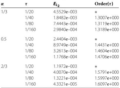
Table 3 The maximumL2errors and convergence orders for Example 2 withh= 1/1,000
α τ EL2 Order(τ)
1/3 1/20 4.5529e–003 ∗
1/40 1.8482e–003 1.3007e+000 1/80 7.4443e–004 1.3119e+000 1/160 2.9840e–004 1.3189e+000
0.5 1/20 2.4404e–003 ∗
1/40 8.9749e–004 1.4431e+000 1/80 3.2613e–004 1.4604e+000 1/160 1.1768e–004 1.4706e+000
2/3 1/20 1.1972e–003 ∗
1/40 4.0070e–004 1.5791e+000 1/80 1.3221e–004 1.5997e+000 1/160 4.3321e–005 1.6097e+000
Table 4 The maximumL2errors and convergence orders for Example 2 withτ= 1/10,000
α h EL2 Order(h)
1/3 1/4 2.9470e–002 ∗
1/8 7.1231e–003 2.0487e+000 1/16 1.7659e–003 2.0121e+000 1/32 4.4129e–004 2.0006e+000
0.5 1/4 2.9634e–002 ∗
1/8 7.1649e–003 2.0482e+000 1/16 1.7757e–003 2.0126e+000 1/32 4.4311e–004 2.0027e+000
2/3 1/4 2.9400e–002 ∗
1/8 7.1113e–003 2.0476e+000 1/16 1.7625e–003 2.0125e+000 1/32 4.3969e–004 2.0031e+000
·
Γ( +α)
Γ( + α)t
+α+
Γ(α)t α–
, <x< , <t≤, ()
u(,t) =t+α+ , u(,t) = –t+α– , <t≤, ()
u(x, ) =cos(πx), ≤x≤. ()
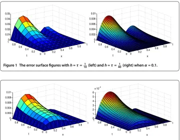
The exact solution isu(x,t) =cos(πx)(t+α+ ). We solve problem ()-() with the Crank-Nicolson-type scheme ()-() and present the numerical results in Tables and . The results show that our scheme is still efficient for nonzero initial value prob-lems. In Figures and , we plot surface figures of the error (|u(xi,tn) –uni|) with different mesh sizes whenα= ., .. These figures show that the maximum error becomes rel-atively smaller as the mesh size becomes smaller, which provides the validation of our results once more.
5 Conclusion
spa-Figure 1 The error surface figures withh=τ=101 (left) andh=τ=401 (right) whenα= 0.1.
Figure 2 The error surface figures withh=τ=101 (left) andh=τ=401 (right) whenα= 0.9.
tial direction. This scheme results in a linear system in which the coefficient matrix is a tridiagonal and strictly diagonally dominant, so it can be solved by the Thomas algorithm. Two numerical examples are given to show the efficiency of the method. It is meaningful to construct a second-order difference scheme of this type, which will be our work in the future.
Competing interests
The authors declare that there is no conflict of interests regarding the publication of this paper.
Authors’ contributions
Both authors contributed equally to the writing of this paper. Both authors read and approved the final manuscript.
Author details
1State Key Laboratory for Geomechanics and Deep Underground Engineering, China University of Mining and
Technology, Xuzhou, Jiangsu 221116, P.R. China.2School of Basic Education Sciences, Xuzhou Medical University, Xuzhou, Jiangsu 221004, P.R. China.3School of Mechanics and Civil Engineering, China University of Mining and Technology, Xuzhou, Jiangsu 221116, P.R. China.
Acknowledgements
We wish to thank the reviewers for their constructive comments that led to the improvement of the original manuscript. Financial support for this work was provided by the National Basic Research Program of China (Nos. 2015CB251601, 2013CB227900), National Natural Science Foundation (Nos. 51322401, 51421003, U1261201), the Fundamental Research Funds for the Central Universities (Nos. 2014YC09, 2014ZDPY08) (China University of Mining and Technology), and the 111 Project (No. B07028).
Received: 23 October 2016 Accepted: 17 January 2017 References
1. Podlubny, I: Fractional Differential Equations. Academic Press, San Diego (1999)
2. Metzler, R, Klafter, J: The random walk’s guide to anomalous diffusion: a fractional dynamics approach. Phys. Rep.339, 1-77 (2000)
4. Zhang, L, Li, S: Regularity of weak solutions of the Cauchy problem to a fractional porous medium equation. Bound. Value Probl.2015, 28 (2015)
5. Povstenko, Y, Klekot, J: The Dirichlet problem for the time-fractional advection-diffusion equation in a line segment. Bound. Value Probl.2016, 89 (2016)
6. Wu, J, Zhang, X, Liu, L, Wu, Y: Twin iterative solutions for a fractional differential turbulent flow model. Bound. Value Probl.2016, 98 (2016)
7. Balakrishnan, V: Anomalous diffusion in one dimension. Physica A132, 569-580 (1985)
8. Schneider, WR, Wyss, W: Fractional diffusion and wave equations. J. Math. Phys.30, 134-144 (1989)
9. Marin, M: Some basic theorems in elastostatics of micropolar materials with voids. J. Comput. Appl. Math.70, 115-126 (1996)
10. Marin, M, Marinescu, C: Thermoelasticity of initially stressed bodies, asymptotic equipartition of energies. Int. J. Eng. Sci.36(1), 73-86 (1998)
11. Hameed, M, Khan, AA, Ellahi, R, Raza, M: Study of magnetic and heat transfer on the peristaltic transport of a fractional second grade fluid in a vertical tube. Eng. Sci. Technol. Int. J.18(3), 496-502 (2015)
12. Langlands, TAM, Henry, BI: The accuracy and stability of an implicit solution method for the fractional diffusion equation. J. Comput. Phys.205, 719-736 (2005)
13. Zhuang, P, Liu, F, Anh, V, Turner, I: New solution and analytical techniques of the implicit numerical method for the anomalous subdiffusion equation. SIAM J. Numer. Anal.46, 1079-1095 (2008)
14. Yuste, SB, Acedo, L: An explicit finite difference method and a new von Neumann-type stability analysis for fractional diffusion equations. SIAM J. Numer. Anal.42, 1862-1874 (2005)
15. Yuste, S: Weighted average finite difference methods for fractional diffusion equations. J. Comput. Phys.216, 264-274 (2006)
16. Sun, ZZ, Wu, XN: A fully discrete difference scheme for a diffusion-wave system. Appl. Numer. Math.56, 193-209 (2006)
17. Lin, X, Xu, C: Finite difference/spectral approximations for the time-fractional diffusion equation. J. Comput. Phys. 225, 1533-1552 (2007)
18. Chen, CM, Liu, F, Turner, I, Anh, V: A Fourier method for the fractional diffusion equation describing subdiffusion. J. Comput. Phys.227, 886-897 (2007)
19. Gao, GH, Sun, ZZ: A compact difference scheme for the fractional subdiffusion equations. J. Comput. Phys.230, 586-595 (2011)
20. Tian, WY, Zhou, H, Deng, WH: A class of second order difference approximations for solving space fractional diffusion equations. Math. Comput.84, 1703-1727 (2015)
21. Li, C, Deng, WH: Second order WSGD operators II: a new family of difference schemes for space fractional advection diffusion equation (2013). arXiv:1310.7671v1 [math.NA]
22. Zhang, YN, Sun, ZZ, Wu, HW: Error estimates of Crank-Nicolson type difference schemes for the subdiffusion equation. SIAM J. Numer. Anal.49, 2302-2322 (2011)
23. Wang, Z, Vong, S: Compact difference schemes for the modified anomalous fractional subdiffusion equation and the fractional diffusion-wave equation. J. Comput. Phys.277, 1-15 (2014)
24. Wang, D, Xiao, A, Yang, W: Crank-Nicolson difference scheme for the coupled nonlinear Schrödinger equations with the Riesz space fractional derivative. J. Comput. Phys.242, 670-681 (2013)
25. Zhao, X, Sun, ZZ: Compact Crank-Nicolson schemes for a class of fractional Cattaneo equation in inhomogeneous medium. J. Sci. Comput.62(3), 747-771 (2014)
26. Sweilam, NH, Moharram, H, Moniem, NKA, Ahmed, S: A parallel Crank-Nicolson finite difference method for time-fractional parabolic equation. J. Numer. Math.22(4), 363-382 (2014)
27. Ozbilge, E, Demir, A: Semigroup approach for identification of the unknown diffusion coefficient in a linear parabolic equation with mixed output data. Bound. Value Probl.2013, 43 (2013)
28. Ozbilge, E, Demir, A: Analysis of the inverse problem in a time fractional parabolic equation with mixed boundary conditions. Bound. Value Probl.2014, 134 (2014)
29. Demir, A, Kanca, F, Ozbilge, E: Numerical solution and distinguishability in time fractional parabolic equation. Bound. Value Probl.2015, 142 (2015)
30. Zhao, X, Xu, Q: Efficient numerical schemes for fractional sub-diffusion equation with the spatially variable coefficient. Appl. Math. Model.38(15-16), 3848-3859 (2014)
31. Vong, S, Lyu, P, Wang, Z: A compact difference scheme for fractional sub-diffusion equations with the spatially variable coefficient under Neumann boundary conditions. J. Sci. Comput.66(2), 725-739 (2015)
32. Metzler, R, Glöckle, WG, Nonnenmacher, TF: Fractional model equation for anomalous diffusion. Physica A211, 13-24 (1994)
33. Zeng, F, Li, C, Liu, F, Turner, I: The use of finite difference/element approaches for solving the time-fractional subdiffusion equation. SIAM J. Sci. Comput.35(6), A2976-A3000 (2013)
34. Sun, ZZ: The Method of Order Reduction and Its Application to the Numerical Solutions of Partial Differential Equations. Science Press, Beijing (2009)