R E S E A R C H
Open Access
Closed-form solutions of transient
electro-osmotic flow driven by AC
electric field in a microannulus
Shaowei Wang
1,2*and Moli Zhao
1,2*Correspondence:
[email protected] 1Department of Engineering
Mechanics, School of Civil Engineering, Shandong University, Jinan, 250061, P.R. China 2Geotechnical and Structural
Engineering Research Center, Shandong University, Jinan, 250061, P.R. China
Abstract
The time-periodic electro-osmotic flow of Newtonian fluids through a microannulus is studied in the Debye-Hückel approximation. Analytical series solutions for velocity and flow rate are presented with the help of an integral transform. The expression for the distribution of the velocity profile consists of a time-dependent oscillating part and a time-dependent generating or transient one, and the normalized velocity function is independent of the Reynolds number, which is very different from previous results. Then the effects of the electrokinetic widthK, the wall zeta potential ratio
β
, and the frequency of applied external electric fieldω
on the distribution of the velocity profiles and flow rates are discussed numerically and theoretically. Some new physical and chemical phenomena are found theoretically. We point out that the electro-osmotic flow driven by an alternating electric field is not periodic in time, but quasi-periodic. There is a phase shift between voltage and flow, which is only dependent on the frequency of the external electric field.Keywords: transient flow; electro-osmosis flow; integral transform; velocity distribution
1 Introduction
When an electric field is applied to the fluids in a channel, the walls of which are charged, the migration of the ions present in excess in the double layer induces the motion of the bulk solution due to viscous drag. This phenomenon provides an attractive means of ma-nipulating liquids in microdevices, and it has been widely used in different microdevices and for various applications, such as microfractionation [, ], electrophoresis [], and microspray generation systems [].
Time-periodic electro-osmotic flow is also known as AC electro-osmosis, and it is driven by an alternating electric field. It is very important for biotechnology and separation sci-ence. Recently, various studies analyzed the time-periodic electro-osmotic flow theory and modeling in different geometry. Dutta and Beskok [] were among the early researchers who analytically investigated the time-periodic electro-osmotic flow between two parallel plates, illustrating interesting similarities or dissimilarities with the Stokes second prob-lem. Based on the method proposed by Dutta and Beskok, many researchers studied time-periodic electro-osmotic flows through microchannels, and some new results are given. General solutions were developed by Xuan and Li [] for direct current and alternating
current electro-osmotic flows in microfluidic channels with arbitrary cross-sectional ge-ometry and arbitrary distribution of wall charge. Jianet al.and his colleagues investigated the flow behavior of time-periodic electro-osmosis in a cylindrical microannulus [, ].
Unfortunately, due to the incorrect critical assumption of the form of velocity distri-bution, the results given in these researches are not correct, and some very important physical phenomena have not been found theoretically. In their researches, these authors believed that the velocity profiles will be oscillatory, and they assumed that these oscilla-tions are instantaneous responses of the externally applied electric fields,i.e., they have the same frequency. True, the electro-osmotic flows should really be generated by the ap-plied time-periodic electric fields, and the flows may be time periodic. But, as we know, there is a phase difference between phase voltage and phase current, and the flow in the microchannel should need some time to start. In other words, there is a phase difference between the applied electric fields and the electro-osmotic flows. On the other hand, on the basis of the aforementioned ‘assumption’, the obtained analytical solutions of velocities are represented as complex functions, which is unreasonable in physics. So, as a result, the solutions given in these research papers are, generally speaking, incorrect.
In fact, the phase shift between the applied electric field and the flow response has been proved by Nayak [], as well as some other researchers []. The steady/unsteady electro-osmotic flow in an infinitely extended cylindrical channel with diameters ranging from to nm has been investigated by Nayak [], and the degree of the phase shift between the velocity field and the applied electric field is found numerically. Using the backwards-Euler time stepping numerical method, Luo [] clarified the relationship between the changes in the axial-flow velocity and the intensity of the applied electric field. Erickson and Li [] developed the analytical solution for the AC electro-osmotic flow through a rectangular microchannel for the case of a sinusoidal applied electric field. Shilovet al.[] discussed the mechanisms for different times after the application of the electrical field according to the relationship between the dipole moment and the electrophoretic mobility.
The aim of the present paper is to present the analytical solutions for the time-periodic electro-osmotic flow of Newtonian fluids through a microannulus. Analytical solutions are rare. Not only do they represent electro-osmotic flows through fundamental cross-sectional shapes but they also serve as standards for asymptotic and fully numerical meth-ods. Most important of all, some new physical and chemical phenomena can be found from the analytical solutions.
2 Governing equations
The motions of an ionized, incompressible Newtonian fluid with electro-osmotic body forces are governed by the following Navier-Stokes equation:
ρDV
Dt = –∇P+μ∇
V+ρ
eE, ()
wherePis the pressure,ρis the fluid density,μis the dynamic viscosity, and the tensorVis a divergence-free velocity field,i.e.,∇ ·V= subject to the non-slip boundary conditions on the walls,E=Ef(t) is the externally applied electric field, andρeis the electric charge
density, which can be expressed by a potential distributionψ; we have
∇ψ= –ρe
and
ρe(r) = –nzvesinh
zveψ(r)
kbT
, ()
herenis the bulk electrolyte concentration of a binary electrolyte dissociating into cations
and anions of valencezv,eis the electron charge,kbis the Boltzmann constant, andTis
the absolute temperature.
In the present study, we assume the surface potential is small enough, then with the help of Debye-Hückel approximation and cylindrical coordinate system (r,θ,z), Eq. () is linearized to
r
∂ ∂r
r∂ψ
∂r
=κψ, ()
whereκ= z
ven/εkbTis the Debye-Hückel parameter and /κmeans the Debye length.
Because of the effect of the electric field, the fluid in the capillary will flow along the axis direction. Neglecting the pressure gradient along the axis, the Cauchy momentum equation in cylindrical coordinate system with AC electric field can be expressed as
ρ∂u ∂t =μ
r
∂ ∂r
r∂u
∂r
+ρe(r)Ecos(ωt), ()
whereu=u(r,t) is the axial velocity,tis time, andEcos(ωt) is AC electric field,Eis the
magnitude, andωis the frequency of the unsteady external electric fieldE.
In the present research, the geometric shape of the microchannel is considered, as shown in Figure . An electrolyte fluid is flowing unsteadily in the annular region between two uniform coaxial circular cylinders with inner radiusRi=αR( <α< ) and outer radius
Ro=R. The chemical interaction of the electrolyte liquid and solid wall generates an
elec-tric double layer (EDL), a very thin charged liquid layer at the solid-liquid interface. The outer and inner wall zeta potentials areψoandψi, respectively. Here,ψoandψiare small
enough, so that the Debye-Hückel linearization approximation is available. Define the following dimensionless variables:
r∗= r
R, t
∗= μt
ρR, ω
∗=ρRω
μ , ψ
∗=zveψ
kbT
, u∗= u
Ueo
, ()
hereUeo= –εkbTE/μzve. Substituting the above dimensionless variables into () and ()
yields the governing equation for the potential distribution with boundary conditions
r
∂ ∂r
r∂ψ
∂r
=Kψ, ()
ψ=ψo∗, r= , ()
ψ=ψi∗, r=α, ()
and the equations for the flow with boundary and initial conditions
∂u
∂t =
r
∂ ∂r
r∂u
∂r
+Kψcos(ωt), ()
u(r,t) = , r=α, ()
u(r,t) = , r= , ()
u(r,t) = , t= . () HereK=κR,ψ∗
i =zveψi/kbTandψo∗=zveψo/kbTare normalized wall potentials. 3 Analytical solutions
The general solution of () has the form
ψ(r) =AI(Kr) +BK(Kr), ()
whereAandBare undetermined constants,I(r) andK(r) are the modified Bessel
func-tions of the first and second kind of order zero, respectively. Considering the boundary conditions () and (), we have
ψ(r) =ψo∗AI(Kr) +BK(Kr)
, ()
and the constantsAandBare
A= K(Kα) –βK(K)
I(K)K(Kα) –I(Kα)K(K)
and
B= I(Kα) –βI(K)
K(K)I(Kα) –K(Kα)I(K)
.
Hereβ=ψi/ψois defined as the ratio of the zeta potentials of the inner wall to that of the
outer wall.
The integral-transform pair in thervariable for the functionT(r,t) is defined as []
˜
T(λm,t) =
α
rR(λm,r)T(r,t)dr, ()
T(r,t) =
∞
m=
R(λm,r) N(λm)
˜
T(λm,t), ()
where
R(λm,r) =J(λmr)Y(λm) –J(λm)Y(λmr), ()
N(λm)
=π
λmJ(αλm) J(αλm) –J(λm)
, ()
andλmis themth positive root ofR(λm,α) = .
Applying the above integral transform () to ()-() yields
˜
ψ(λm) =
ψo∗ π(λ
m+K)
–β J(λm)
J(αλm)
, ()
du˜ dt = –λ
mu˜+Kψ˜cos(ωt), ()
˜
u(λm,t) = , t= . ()
Equation () is an ordinary differential equation with initial condition (), and its so-lution can be given directly as
˜
u(λm,t) =Kψ˜(λm)
sin(ωt+Φm)
λ
m+ω
– λ
m
λ
m+ω e–λmt
, ()
whereΦm=arctan(λm/ω) <π/ is the phase difference or the phase shift, andψ˜(λm) can
be obtained from () with the help of the aforementioned integral transform (). Then, substitutingψ˜(λm) into Eq. () yields the distribution of the velocity in the capillary,
u(r,t) =K
∞
m=
π λmJ(αλm)[J(λmr)Y(λm) –J(λm)Y(λmr)]
(λ
m+K)[J(αλm) –J(λm)]
×
ψo∗–ψi∗ J(λm)
J(αλm)
sin(ωt+Φm)
λ
m+ω
– λ
m
λ
m+ω e–λmt
. ()
4 Results and discussion 4.1 The generation of the flow
From the expression (), we find that the velocity field of electro-osmotic flow in the capillary generated by the external applied electric field is not time periodic. In particu-lar, the distribution of the velocityu(r,ϕ,t) can be written as a sum of a time-dependent oscillating partu(r,t) and a time-dependent generating partu(r,t):
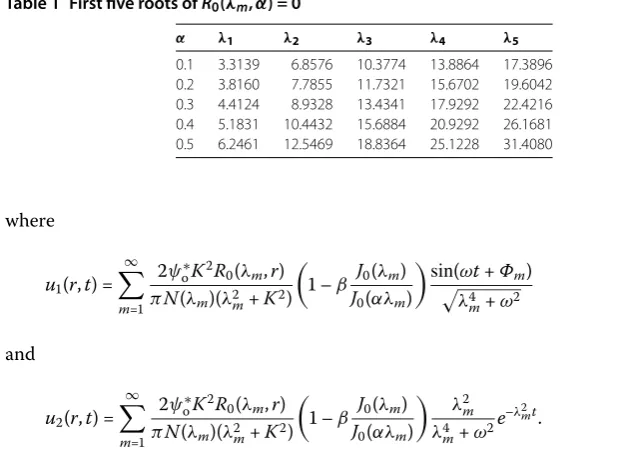
Table 1 First five roots ofR0(λm,α) = 0
α λ1 λ2 λ3 λ4 λ5
0.1 3.3139 6.8576 10.3774 13.8864 17.3896 0.2 3.8160 7.7855 11.7321 15.6702 19.6042 0.3 4.4124 8.9328 13.4341 17.9292 22.4216 0.4 5.1831 10.4432 15.6884 20.9292 26.1681 0.5 6.2461 12.5469 18.8364 25.1228 31.4080
where
u(r,t) = ∞
m=
ψo∗KR (λm,r)
πN(λm)(λm+K)
–β J(λm)
J(αλm)
sin(ωt+Φm)
λ
m+ω
()
and
u(r,t) = ∞
m=
ψo∗KR (λm,r)
πN(λm)(λm+K)
–β J(λm)
J(αλm)
λ
m
λ
m+ω
e–λmt. ()
HereR(λm,r) andN(λm) are defined by () and (), respectively.
The first five roots ofR(λm,α) = for differentαare listed in Table . It can be seen
that the minimum ofλm increases with increasingα. Whenα= ., for the minimum of
λmwe haveλ=min{λm} ., ande–λ
.×–. As a result, we can draw the
con-clusion that the generating part of the solution () will tend to zero in a very short time, which results in the electro-osmotic flow reaching a steady ‘periodic’ state. Additionally, it is worth pointing out that the increasing frequency of the applied external electric field accelerates the generation of flow in the microannulus.
In the sense of the above discussion, the generating part can also be called the tran-sient part. In other words, the electro-osmotic flow generated by the AC electric field is quasi-periodic. In spite of this, the generating part of the solution is very important for the researcher in this field, since it explains both the characteristics of electro-osmotic flow and the practical applications due to rapid development of the biochip technology []. Furthermore, in a study of the stability of a colloidal system, Overbeek [] pointed out that the relaxation time for surface charges (about – to s) and the time scale for Brownian coagulation (about –to –s) are very different; the aggregation of colloidal
particles may occur earlier than the equilibrium of the electrical conditions near a surface. In these cases, the steady-state analysis on the electrical condition near a charged surface is unrealistic, and an extension of the conventional treatment to a temporal description is inevitable, and this is the significance of the present study.
4.2 Special cases
In particular, whenω→,i.e.,E(t) =EH(t), whereH(t) is the Heaviside step function,
lim ω→arctan
λ ω = π , () which yields lim
Then we get the distribution of velocity profile when the applied external electric field remains constant from timet= ,i.e., the electric field follows a step-change:
u(r,t) =K
∞
m= π λ
mJ(αλm)[J(λmr)Y(λm) –J(λm)Y(λmr)]
(λ
m+K)[J(αλm) –J(λm)]
×
ψo∗–ψi∗ J(λm)
J(αλm)
–e–λmt. ()
Whenβ= , then we haveψo∗=ψi∗,i.e., the inner wall and outer one have the same zeta potential,
u(r,t) =ψo∗K
∞
m=
π λmJ(αλm)R(λm,r)
(λ
m+K)[J(αλm) +J(λm)]
×
sin(ωt+Φm)
λ
m+ω
– λ
m
λ
m+ω e–λmt
. ()
Whenβ= ,ψi∗= ,i.e., the inner wall is not charged, then the solution of velocity () reduces to
u(r,t) =ψo∗K
∞
m= π λmJ
(αλm)[J(λmr)Y(λm) –J(λm)Y(λmr)]
(λ
m+K)[J(αλm) –J(λm)]
×
sin(ωt+Φm)
λ
m+ω
– λ
m
λ
m+ω e–λmt
. ()
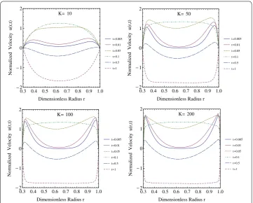
4.3 Effects ofKon velocity profiles and flow rates
For given values α = .,ω= ,ψo = , andβ = , plots of the normalized velocity
u(r,t)/Ueo as a function of the non-dimensional radiusr/Rfor selected values of timet
and for four different values of the electrokinetic widthKare shown in Figure . It is clear from this figure that the flow in the microannulus is similar to general pipe flow for small
Kas shown in the figure whenK= , because the EDL is thicker for smallK. When the value ofKis large enough, the velocity of the flow increases with increasing electrokinetic widthK, and this phenomenon can also be proved analytically from the expression (), where the termK/(λ
m+K) is included. The same conclusion is true for the flow rate of
fluid, which can be obtained by integrating Eq. (),
Q(t) =K
∞
m=
πλmJ(αλm)
(λ
m+K)[J(αλm) –J(λm)]
ψo∗–ψi∗ J(λm)
J(αλm)
×Y(λm)
J(λm)αJ(αλm)
–J(λm)
Y(λm) –αY(αλm)
×
sin(ωt+Φm)
λ
m+ω
– λ
m
λ
m+ω e–λmt
. ()
To demonstrate the effect of K on the flow rate, plots of the flow rate as a function of
Figure 2 Effects ofKon the distribution of velocity profiles at different times:K= 10, 50, 100, 200.
Figure 3 Effects ofKon flow rate at differentω:ω= 0, 10.
Additionally, some authors drew the conclusion that the flow rate is proportional to the cross-sectional area of the channel for largeK, and the flow rate is quadratic asKin the
leading-order behavior for smallK[–]; it is noteworthy that this conclusion is incor-rect. In this research, the authors discussed the asymptotic expansion ofK/(λm+K) for large and smallK, respectively, with the help of series summation formulas. Unfortu-nately, they ignored the fact that{λm}is a monotonically increasing infinite subsequence.
In other words, for a givenK, no matter how large it is, there exists a natural numberN
On the other hand, from Figure and Eqs. ()-(), it is important to note that because the transient part of the velocity solution decays in a short time, if the researchers consider the electro-osmotic flow of fluids for timet> , the time-dependent oscillating partu(r,t)
can be used as a good approximation for simplicity of computation.
4.4 Effects of
ω
on velocity profilesFigure indicates the axial velocity distributions along the axial direction during the pe-riod of transient response fromt= tot= for different values ofω. For givenα= .,
K= ,ψo= , andβ= , the oscillation of flow is enhanced by the increasing frequency
of the applied external electric field. However, the mean velocity of flow decreases asω in-creases fromω= toω= ,. An interesting phenomenon is found: there is almost no flow in the areas far away from the EDL whenωis large enough, as in the case ofω= ,.
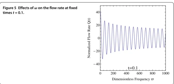
Figure 5 Effects ofωon the flow rate at fixed timest= 0.1.
As the frequency of external electric field increases, the flow rate gets closer to zero, and it keeps its oscillation, as shown in Figure , which is obtained from () as a function of
ωat fixedt= .. The physical interpretation is that the large frequency AC electric field makes the ions in the fluid oscillate around an equilibrium position. Mathematically and analytically, the increasingωdecreases the term in Eq. (),
sin(ωt+Φm)
λ
m+ω
– λ
m
λ
m+ω
e–λmt; ()
as a result, the velocity reliably decreases with increasing frequency of the applied external electric field. Away from the walls of the microannulus, the EDL can be divided into the compact layer and the diffuse double layer. Within the diffuse layer, the motion of the ions is subject to the zeta potential of the EDL. Then we have the conclusion that the main contribution to the flow rate is the zeta potential when the frequency of the applied AC electric field is large enough.
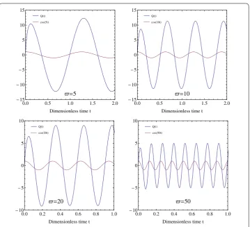
Additionally, the effects ofωon the normalized flow rate and phase shift are shown in Figure for givenK= . With the increasing frequency of the applied external electri-cal field, there appears to be a decrease of the phase shift between voltage and flow. In fact, according to Eq. (),φmmathematically tends to be zero for large enoughω. At the
same time, Figure shows the increasing frequency decreases the flow rateQ(t), which is consistent with the results shown in Figure and Figure .
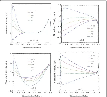
4.5 Effects of wall zeta potential ratio
β
on velocity profilesFigure 6 Effects ofωon the flow rate and phase shift:ω= 5, 10, 20, 50.
the microannulus,i.e.,u(t) =Q(t)/π, and the following relationship is obtained:
u(t)∼ –β J(λm)
J(αλm)
. ()
5 Summary and conclusion
Figure 7 Effects ofβon the distribution of velocity profiles at different times:t= 0.05, 0.1, 0.5, 1.
Competing interests
The authors declare that they have no competing interests.
Authors’ contributions
All authors contributed equally to the writing of this paper. All authors read and approved the final manuscript.
Acknowledgements
This work is supported by the National Natural Science Foundation of China (Nos. 11002083, 51279093), the National Basic Research Program of China (2013CB0360000).
Received: 9 June 2014 Accepted: 9 September 2014
References
1. Effenhauser, CS, Manz, A, Widmer, HM: Manipulation of sample fractions on a capillary electrophoresis chip. Anal. Chem.67, 2284-2287 (1995)
2. Raymond, DE, Manz, A, Widmer, HM: Continuous separation of high molecular weight compounds using a microliter volume free-flow electrophoresis microstructure. Anal. Chem.68, 2515-2522 (1996)
3. Harrison, DJ, Manz, A, Fan, ZH, Ludi, H, Widmer, HM: Capillary electrophoresis and sample injection systems integrated on a planar glass chip. Anal. Chem.64, 1926-1932 (1992)
4. Ramsey, RS, Ramsey, JM: Generating electrospray from microchip devices using electroosmotic pumping. Anal. Chem.69, 1174-1178 (1997)
5. Dutta, P, Beskok, A: Analytical solution of time periodic electroosmotic flows: analogies to Stokes’ second problem. Anal. Chem.73, 5097-5102 (2001)
6. Xuan, X, Li, D: Electroosmotic flow in microchannels with arbitrary geometry and arbitrary distribution of wall charge. J. Colloid Interface Sci.289, 291-303 (2005)
7. Jian, Y, Yang, L, Liu, Q: Time periodic electro-osmotic flow through a microannulus. Phys. Fluids22, 042001 (2010) 8. Bao, LP, Jian, YJ, Chang, L, Su, J, Zhang, HY, Liu, QS: Time periodic electroosmotic flow of the generalized Maxwell
fluids in a semicircular microchannel. Commun. Theor. Phys.59, 615-622 (2013)
10. Luo, WJ: Transient electroosmotic flow induced by DC or AC electric fields in a curved microtube. J. Colloid Interface Sci.278, 497-507 (2004)
11. Erickson, D, Li, D: Analysis of alternating current electroosmotic flows in a rectangular microchannel. Langmuir19, 5421-5430 (2003)
12. Shilov, VN, Delgado, AV, González-Caballero, F, Horno, J, López-García, JJ, Grosse, C: Polarization of the electrical double layer. Time evolution after application of an electric field. J. Colloid Interface Sci.232, 141-148 (2000) 13. Özisik, MN: Heat Conduction, 2nd edn. Wiley, New York (1993)
14. Wong, PK, Chen, C, Wang, T, Ho, C: Electrokinetic bioprocessor for concentrating cells and molecules. Anal. Chem.76, 6908-6914 (2004)
15. Overbeek, JTG: Recent developments in the understanding of colloid stability. J. Colloid Interface Sci.58, 408-422 (1977)
16. Wang, CY, Liu, YH, Chang, CC: Analytical solution of electro-osmotic flow in a semicircular microchannel. Phys. Fluids
20, 063105 (2008)
17. Wang, CY, Chang, CC: EOF using the Ritz method: application to superelliptic microchannels. Electrophoresis28, 3296-3301 (2007)
18. Chang, CC, Kuo, CY, Wang, CY: Unsteady electroosmosis in a microchannel with Poisson-Boltzmann charge distribution. Electrophoresis32, 3341-3347 (2011)
doi:10.1186/s13661-014-0215-2