A collocation spectral method for two-dimensional Sobolev equations

R E S E A R C H

Open Access

A collocation spectral method for

two-dimensional Sobolev equations

Shiju Jin

_{and Zhendong Luo}

*_{Correspondence: [email protected]}

2_{School of Mathematics and}

Physics, North China Electric Power University, Beijing, China Full list of author information is available at the end of the article

Abstract

This article mainly studies a collocation spectral method for two-dimensional (2D) Sobolev equations. To this end, a collocation spectral model based on the Chebyshev polynomials for the 2D Sobolev equations is first established. And then, the existence, uniqueness, stability, and convergence of the collocation spectral numerical solutions are discussed. Finally, some numerical experiments are provided to verify the

corrections of theoretical results. This implies that the collocation spectral model is very effective for solving the 2D Sobolev equations.

MSC: 65N30; 65N12; 65M15

Keywords: Collocation spectral method; Sobolev equation; Existence and stability as well as convergence; Numerical experiment

1 Introduction

Because any bounded closed domain inR2 _{can be approximately filled with several} rectangles [ai,bi]×[ci,di] (i= 1, 2, . . . ,I), for convenience and without losing universality, let us just assume that= [a,b]×[c,d]⊂R2_{, whose boundary is denoted by∂, consider} the following two-dimensional (2D) Sobolev equations:

⎧ ⎪ ⎪ ⎨ ⎪ ⎪ ⎩

ut–εut–γ u=f(x,y,t), (x,y,t)∈×[0,T],

u(x,y,t) =ϕ(x,y,t), (x,y,t)∈∂×[0,T],

u(x,y, 0) =u0(x,y), (x,y)∈,

(1)

whereut=∂u/∂t,u=∂2_u/∂x2_+∂2_u/∂y2_,ut=∂2_ut/∂x2_+∂2_ut/∂y2_{,Tis the total time,ε} andγ are two given positive constants,f(x,y,t) is given source term,u0(x,y) andϕ(x,y,t) are initial and boundary value functions, respectively. For the sake of convenience, but without loss of generality, we assumeϕ(x,y,t) = 0 in the following analysis.

The Sobolev equations hold very significant physical background so that they have be-come a class of important evolution partial differential equations (PDEs) and have been successfully used to many numerical simulations in mathematical and physical problems, such as the exchange in different media (see [1]) and the moisture migration in soil (see [2]). In particular, the Sobolev equations can be used to depict the porous phenomena saturated into rocks with cracks (see [3, 4]). However, the Sobolev equations in the

world problems usually include the complex known data, such as the complicated initial and boundary value conditions, or the intricate source term, or the discontinuous coef-ficients, so that they have no analytic solution. Thus, they have to depend on numerical solutions.

At present, finite difference scheme (FDS), finite element method (FEM), finite volume element method (FVEM), and spectral method are considered to be four well-known nu-merical methods. By comparison, the spectral method can attain higher accuracy be-cause it adopts Fourier and orthogonal polynomials to approximate unknown function, but other numerical methods use ordinary polynomials or difference quotient. Especially, with the rapid development of the electronic computers, the spectral method has achieved great success in many applied fields (see, e.g., [5, 6]). The spectral method is a weighted residual way for PDEs and is usually classified as the Galerkin spectral method, the collo-cation spectral method (CSM), and the spectral element method, which are used to solve the second-order elliptic, parabolic, hyperbolic, hydromechanics PDEs, and so on (see [4– 10]).

Although FDS, FEM, and FVEM have been used to solve the Sobolev equations (see [3, 4, 10–13]), the spectral method, especially CSM, has yet not been used to solve the 2D Sobolev equations, except a Fourier spectral method has been used to solve the one-dimensional Sobolev equations in [14]. Therefore, in this article, we first develop a CSM for the 2D Sobolev equations. And then, we provide the existence, uniqueness, stability, and convergence for its CSM solutions. Finally, we give some numerical experiments to verify the correctness of theoretical results. Moreover, it is shown that the CSM scheme is very effective for solving the 2D Sobolev equations.

The rest of this article is arranged as follows. In Sect. 2, we first review the basic theory of spectral-collocation method and some Sobolev spaces. And then, in Sect. 3, we build the CSM scheme for the 2D Sobolev equations and analyze the existence, uniqueness, stability, and convergence of the CSM solutions. Next, in Sect. 4, we use some numerical experiments to verify that the results of numerical computations accord with the theoreti-cal analysis and to certify that the CSM scheme is very efficient for solving the 2D Sobolev equations. Finally, we offer the main conclusions and discussion in Sect. 5.

2 The basic theory of CSM and some Sobolev spaces 2.1 The basic theory of spectral-collocation method

The rationale of the spectral methods is to approximate the solutionuof PDE with a fi-nite sumuN. In CSM, the approximate functionuN ∈PN is denoted by its values at the Gauss-type interpolation points. In this study, we shall adopt the more common points, i.e., the so-called Chebyshev–Gauss–Lobatto (CGL) points (see [6]), as the interpolation nodes.

The Chebyshev polynomials are some special Jacobi polynomials, which are orthogonal with the Chebyshev weight functionω(x) = 1/√1 –x2_{over [–1, 1], namely}

1 –1

Tm(x)Tn(x)ω(x) dx=γnδm,n,

whereγn=Tn2ω=

1

Let{xj}N_j=0and{yk}N_k=0be two sets of space nodes, i.e., the CGL points inxandy direc-tions, respectively, and{ωk}N_k=0 be a set of weights. Then they are, respectively, defined by

xk= –cosπk

N , yk= –cos kπ

N , ωk= π ckN

, 0≤k≤N, (2)

wherec0=cN = 2 andck= 1 (k= 1, 2, . . . ,N– 1). They hold the following property (see, e.g., [5]).

Theorem 1 Let {xk}N

k=0, {yk}Nk=0, and{ωk}Nk=0 be the sets of CGL quadrature nodes and

weights,respectively.Then there holds

1 –1

1 –1

p(x,y)ω(x)ω(y) dxdy=

N

j=0

N

k=0

p(xj,yk)ωjωk, ∀p(x,y)∈P2N–1. (3)

The fundamental of CSM is to get an approximation solution foru(x,y) by a sum

uN(x,y) =

N

j=0

N

k=0

uN(xj,yk)hj(x)hk(y), (4)

whereuN(x,y)∈PN, the interpolation nodes{xj}N

j=0and{yk}Nk=0are the CGL points given by (2), and{hj(x)}N_j=0and{hk(y)}N_j=0are the Lagrange basis polynomials associated with the sets of the CGL points{xj}N_j=0and{yk}N_k=0, respectively.

Moreover, the derivative ofuN(x,y) atxkis denoted by

∂uN(xk,y)

∂x = N

j=0

N

l=0

uN(xj,yl)h

j(xk)hl(y), 0≤k≤N. (5)

The first-order derivative ofhj(x) at the CGL points can be denoted by the following ex-plicit formulas:

h_j(xk) =

⎧ ⎪ ⎪ ⎪ ⎪ ⎪ ⎪ ⎨ ⎪ ⎪ ⎪ ⎪ ⎪ ⎪ ⎩

–2N2+1

6 , k=j= 0,

ck

cj (–1)k+j

xk–xj , k=j, 0≤k,j≤N, – xk

2(1–x2_k), 1≤k=j≤N– 1, 2N2₊₁

6 , k=j=N,

(6)

wherec0=cN = 2 andck= 1 (k= 1, 2, . . . ,N– 1). By replacingxin (5) and (6) withy, we easily obtain the computational approach of∂uN(x,yk)/∂y.

2.1.1 Some useful Sobolev spaces

Let∈Rn_{(n= 1, 2) be a bounded open domain with boundary∂, and letL}2_{() denote} the set of all square-integrable functions defined on.

For a non-negative integer m, and α = (α1,α2, . . . ,αn) (αi≥0 are integer and |α|= n

i=1αi), define

Hm() =u∈L2() :Dαu∈L2(), 0≤ |α| ≤m,

equipped with the norm and semi-norm as follows, respectively:

um=

0≤|α|≤m

Dαu2₀

1/2

, |u|m=

|α|=m

Dαu2₀

1/2 .

SetHm

0() ={u∈Hm() :Dαu(x)|∂= 0,|α|<m}andH–m() denotes the dual space of

H₀m().

Further, letω=:ω(x,y) =ω(x)ω(y) = 1/(1 –x2_{)(1 –y}2_{),= (–1, 1)}2_,L2

ω() denote the

set of all square-integrable functions defined on, equipped with the norm

u0,ω=

|u|2_ωd

1/2 ,

andHm

ω() :={u∈L2ω() :Dαu∈L2ω(), 0≤ |α| ≤m}be a weighted Sobolev space on

with the CGL quadrature weight function, equipped with the norm

um,ω=

0≤|α|≤m

Dαu2_0,ω

1 2

, u0,ω=

|u|2_ωd

1 2

, ω=ω(x)ω(y).

Furthermore, setH1

0,ω() ={u∈Hω1() :u|∂= 0}, (·,·)ωdenotes the weighted inter

prod-uct ofL2

ω() =Hω0(), and · Hl(Hωm)is the norm in the following space:

Hl0,T;H_ωm()≡

v(t)∈H_ωm() :v2_Hl_(Hm

ω)≡

T

0

l

i=0

_dd_tiiv(t)

2

m,ω

dt<∞

.

Next, define theHω1-orthogonal projectionRN :H0,1ω()→PN such that, for anyu∈

H1

0,ω(), there holds

∇(RNu–u),∇v_ω= 0, ∀v∈PN,

where= [–1, 1]2_{and (·,·)}

ωis the inner product inL2ω()2about the Chebyshev weight

functionω=ω(x,y) =ω(x)ω(y) = 1/(1 –x2_{)(1 –y}2_{), or equivalently,}

uN(x,y) =RNu(x,y) = N

j=0

N

k=0

uN(xj,yk)hj(x)hk(y). (7)

Therefore, we can also approximate the unknown solutionu(x,y) withRNu(x,y). In

Theorem 2 For any u∈Hωq()with q≥2,we have

∇RNu0,ω≤ ∇u0,ω, ∂k(RNu–u)_0,ω=O

Nk–q, 0≤k≤q≤N+ 1.

Finally, we provide several formulas used often in the following discussions.

(1) The Poincaré inequality

There exists a constantCpsuch that

Cpum≤ |u|m≤ um, ∀u∈H₀m().

(2) The Hölder inequality

|uv|d≤

|u|2_d

1

2

|v|2_d

1 2

, ∀u,v∈L2().

(3) Green’s formula

vud= –

∇u· ∇vd+

∂

v∂u

∂nds, ∀u∈H

2_(),∀v∈H1_(),

whereu= n_i=1∂2_u/∂x2

i,∇u= (∂u/∂x1,∂u/∂x2, . . . ,∂u/∂xn), andnis the unit outer normal vector on∂.

(4) The Cauchy inequality

ab≤εa

2

2 +

b2

2ε, ∀a≥0,b≥0,ε> 0.

3 CSM for the 2D Sobolev equations

3.1 The variational formulation for the 2D Sobolev equations

By Green’s formula, we can attain the following variational formulation for the 2D Sobolev equations (1).

Problem 3 Fort∈(0,T), findu∈H1

0,ω() such that

⎧ ⎨ ⎩

(ut,v)ω+ε(∇ut,∇v)ω+γ(∇u,∇v)ω= (f,v)ω, ∀v∈H0,1ω(),

u(x,y, 0) =u0(x,y), (x,y)∈.

(8)

For Problem 3, we have the following result of the existence, uniqueness, and stability of the generalized solution.

Theorem 4 If f ∈L2_(0,T;L2

ω())and u0∈Hω1(),then there exists a unique generalized

solution for the variational formulation(8)satisfying the following stability:

u1,ω≤ ˜c

u01,ω+f_L2_(L2 ω)

, (9)

wherec˜=max{1,ε, 1/(γC2

Proof Because (8) is a system of linear equations about unknown functionu, to demon-strate that there exists a unique solution for the variational formulation (8) is equivalent to proving that equation (8) has only a zero solution whenf(x,y,t) =u0(x,y) = 0.

Takingv=uin the first formula of equation (8), we have

du2_0,ω

2 dt +ε

d∇u2_0,ω

2 dt +γ∇u

2

0,ω= (f,u)ω. (10)

By integrating (10) from 0 tot∈[0,T] and by the Hölder, Poincaré, and Cauchy inequali-ties, we obtain

u2

0,ω+ε∇u20,ω+ 2γ

t

0

∇u2 0,ωdt

=u020,ω+ε∇u020,ω+ 2

t

0

(f,u)ωdt

≤ u020,ω+ε∇u020,ω+

1

γC2

p

t

0

f2_0,ωdt+γ

t

0 ∇

u2_0,ωdt. (11)

Therefore, whenf(x,y,t) =u0(x,y) = 0, we obtainu0,ω=∇u0,ω= 0, which impliesu=

0, namely the variational formulation (8) has a unique solutionu∈H_0,1ω(). Further, from

(11), we obtain (9). This completes the proof of Theorem 4.

3.2 CSM for the 2D Sobolev equations

When solving time-dependent PDEs by CSM, we use FDS in time and the spectral method in space. In the following discussions, for convenience, we can assume a=c= –1 and

b =d= 1 because, by employing transforms x = –1 + 2(x–a)/(b–a) and y= –1 + 2(y–c)/(d–c), we can ensure [a,b]↔[–1, 1] and [c,d]↔[–1, 1], respectively.

3.2.1 Establishment of the CSM scheme

The main idea of CSM is to seek an approximate solution at time and spatial nodes. In this article, we will take the CGL type interpolation points as the space nodes. Namely, let

{xj}N

j=0and{yk}Nk=0be the space nodes inxandydirections, respectively, with

xj= –cosjπ

N, yk= –cos kπ

N,

where the positive integerNdenotes the number of nodes in a certain direction. And, for integerK> 0, lett=T/K be the time step, i.e.,Kt=T. We approximateu(x,y,nt) withun_{, the time derivativeutofu(x,y,t) at timetn=ntwith (u}n+1_–un_{)/t, andu}n_(x,y)

withun_N(x,y), namely

un(x,y)≈un_N(x,y) =

N

j=0

N

k=0

un_N(xj,yk)hj(x)hk(y), 0≤n≤K.

Problem 5 Findun_N∈UN ≡H1

0,ω()∩PN such that

⎧ ⎪ ⎪ ⎨ ⎪ ⎪ ⎩

(un+1

N –unN,vN)ω+ε(∇un_N+1–∇u_Nn,∇vN)ω+γ t(∇un_N+1,∇vN)ω

=t(f(tn+1),vN)ω, ∀vN∈UN, 0≤n≤K,

u0

N(x,y) =RNu0(x,y), (x,y)∈,

(12)

wheref(tn) =f(x,y,tn).

3.2.2 Existence,uniqueness,and stability of the CSM solutions

For Problem 5, we have the result of the existence, uniqueness, and stability about the CSM solutions.

Theorem 6 If f ∈L2(0,T;L2ω())and u0∈Hω1(),then there exists a unique series of

so-lutions un

N∈UN (n= 1, 2, . . . ,K)for the CSM scheme(12)satisfying the following stability:

_∇un_N0,ω≤ ∇u00,ω+

t γ n j=1

f(tj)

2 0,ω

1/2

, n= 1, 2, . . . ,K. (13)

Proof Because scheme (12) is a linear system of equations aboutun_N+1, in order to demon-strate the existence and uniqueness of solutions for the CSM scheme (12), it is necessary to prove that (12) has only zero solution whenu0(x,y) =f(x,y,t) = 0.

By takingvN=un+1

N –unN in the first equation of (12), we have

un_N+1–un_N2_0,ω+ε∇un_N+1–∇un_N2_0,ω+γ t∇un_N+12_0,ω

=γ t∇un_N+1,∇un_N0,ω+tf(tn+1),unN+1–unN

0,ω. (14)

Then, by the Hölder and Cauchy inequalities, we obtain

un_N+1–un_N2_0,ω+ε∇un_N+1–∇un_N2_0,ω+γ t∇un_N+12_0,ω

≤γ t

2 ∇u

n+1

N

2 0,ω+

γ t

2 ∇u

n N

2 0,ω+

t2

2 f(tn+1) 2 0,ω+

1 2u

n+1

N –unN

2

0,ω. (15)

By summing (15) from 1 tonand using the second formula of (12), we obtain

n

j=0

uj_N+1–uj_N2_0,ω+ 2ε n

j=0

_∇uj+1

N –∇u j N

2

0,ω+γ t∇u

n+1

N

2 0,ω

≤γ t∇u020,ω+t2

n

j=0

f(tj+1) 2

0,ω, n= 0, 1, 2, . . . ,K– 1. (16)

Thus, from (16), we obtain∇un+1

N ω= 0 (n= 0, 1, . . . ,K– 1) whenf =u0= 0, which im-pliesun_N = 0 (n= 1, 2, . . . ,K). In other words, the CSM scheme (12) has a unique series of solutions. From (16), we immediately attain (13). This completes the proof of

3.2.3 The convergence of the CSM solutions

For the series of solutions of Problem 5, we have the following conclusion of conver-gence.

Theorem 7 Under the same conditions of Theorem6,if the solutions of Problem3u(tn)∈

Hωq() (2≤q≤N+ 1),whent=O(N–1),the errors between the solution for Problem3

and the series of solutions of Problem5have the following estimates:

_∇

u(tn) –unN0,ω=O

t,N1–q_{, 1≤n≤K, 2≤q≤N+ 1. (17)}

Proof Leten

1=u(tn) –un,en2=un–RNun, anden3=RNun–unN.

(1) First, estimateen₁.

If we adopt (un+1_–un_{)/tto approximateu}

t, we obtain the following semi-discretize

formulation of equation (8) about time:

1

t

un+1–un,v_ω+ ε

t

∇un+1_–∇un_,∇v

ω+γ

∇un+1,∇v_ω =f(tn+1),v

ω, ∀v∈H

1

0,ω(). (18)

At timet=tn, by applying Taylor’s expansion to (8) and subtracting (18), takingv=en1+1–

en₁, we obtain

en₁+1–en₁2_0,ω+ε∇e₁n+1–en₁2_0,ω+γ t∇en₁+12_0,ω

=t 2

2

utt

ξ₁n,en₁+1–en_1ω

+εt 2

2

∇utt

ξ₂n,∇e₁n+1–en_1ω

+γ t∇en₁+1,∇en_1ω, (19)

wheretn≤ξ₁n,ξ₂n≤tn+1. By using the Hölder and Cauchy inequalities, we obtain

en₁+1–en₁2_0,ω+ε∇e₁n+1–en₁2_0,ω+γ t∇en₁+12_0,ω

≤1 2 t2 2 2

uttξ₁n2

0,ω+

1 2e

n+1 1 –en1

2 0,ω +ε 2 t2 2 2

_∇uttξ₂n2_0,ω

+ε 2∇

en₁+1–en₁2_0,ω+γ t 2 ∇e

n+1 1

2 0,ω+∇e

n 1 2 0,ω . (20)

Further, we obtain

γ t∇en₁+12_0,ω≤t

4

4 ut

ξ₁n2

0,ω+

εt4

4 ∇utt

ξ₂n2

0,ω

Ase0₁= 0, by summing (21) from 0 ton, we obtain

_∇en+1 1

2 0,ω≤

t3 4γ

n

j=0

utξ1j2_0,ω+ε∇utt

ξ2j2_0,ω

,

namely

_∇en₁+1_0,ω≤Ct, 0≤n≤K– 1, (22)

whereC2₌t

4γ

n

j=0(utt(ξ1n)20,ω+εutt(ξ2n)20,ω).

(2) Next, estimatee2.

The estimate ofe2can be immediately obtained by Theorem 2, i.e.,

_∇en

20,ω=O

N1–q, n= 1, 2, . . . ,K, 2≤q≤N+ 1. (23)

(3) Finally, discuss the estimate ofe3=RNun–unN.

By subtracting Problem 5 from (18) takingv=vN∈UN, we obtain

un+1–un_N+1–un–un_N,vN_ω+γ t∇un+1–un_N+1,∇vN_ω

+ε∇un+1–un_N+1–un–un_N,∇vN

ω= 0, ∀vN∈UN. (24)

By Theorem 2, (24), the property ofRN, and the Hölder and Cauchy inequalities, we

have

en₃+1–en₃2_0,ω+ε∇e₃n+1–en₃2_0,ω+γ t∇en₃+12_0,ω

=un+1–un–un_N+1–un_N,en₃+1–en₃

+RNun+1–un+1–RNun–un,en₃+1–en₃

+ε∇un+1–un_N+1–un–un_N,∇en₃+1–en₃

+ε∇RNun+1–un+1–

RNun–un

,∇en₃+1–en₃

+γ t∇RNun+1–un+1

,∇en₃+1–en₃

+γ t∇un+1–u_Nn+1,∇en₃+1–en₃

=RNun+1–un+1–RNun–un,en₃+1–en₃ ≤1

2e

n+1 3 –en3

2

0,ω+RNu

n+1_–un+12

0,ω+RNu

n_–un2 0,ω

≤1

2e

n+1 3 –en3

2 0,ω+CN

–2q_{, n= 0, 1, . . . ,K– 1, 2≤q≤N+ 1. (25)}

Whent=O(N–1_{), from (25), we attain}

_∇en

30,ω=O

N–q–1/2, n= 1, 2, . . . ,K, 2≤q≤N+ 1. (26) By combining (22)–(23) with (26), we attain (17). This completes the proof of

By using the Nietzsche technique and Theorem 7, we easily obtain the followingL2

ω

norm error estimates.

Corollary 8 Under the same conditions of Theorem6,whent=O(N–1_{),the L}2

ωnorm

error estimates between the solution for Problem3and the series of solutions of Problem5

are as follows:

u(tn) –un_N0,ω=Ot2,N–q, 1≤n≤K, 2≤q≤N+ 1. (27)

Remark1 The error estimates in Theorem 7 and Corollary 8 attain an optimal order be-cause one can only ensureu∈H1(0,T;Hω2()) whenf ∈L2(0,T;L2ω()) andu0∈Hω1().

Theorem 6 shows that the CSM scheme, i.e., Problem 5 for the 2D Sobolev equations, has a unique series of solutions which is stable and continuously depends on the initial value and source functions. This theoretically ensures that Problem 5 is effective and reliable for solving the 2D Sobolev equations.

4 Numerical experiments

In this section, we give some numerical experiments to verify the correction of the theo-retical results of the CSM scheme, i.e., Problem 5 for the 2D Sobolev equations.

In the 2D Sobolev equation (1), we took¯ = [–1, 1]×[–1, 1],ε= 1/π2,γ= 2/π2,ϕ= 0,

u0(x,y) = 1 –cos2πxcos2πy, andf(x,y,t) = 2(cos2πxcos2πy– 1)exp(–2t). Thus, we can find the analytical solutions for the Sobolev equations (1) as follows:

u(x,y,t) = (1 –cos2πxcos2πy)exp(–2t), (x,y,t)∈[–1, 1]×[–1, 1]×[0,∞).

When we take time step t= 0.01 and the number of nodes in every directionN= 100, from Corollary 8, the theoretical errors between the analytical solution and the CSM solutionsuk

N (k= 1, 2, . . . ,K) should beO(10–4).

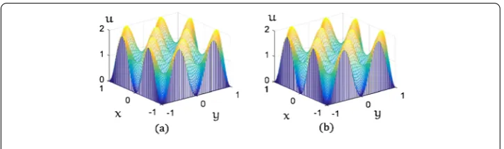
By the CSM scheme (12), we obtained the CSM numerical solutions atT= 0, 0.3, 0.5, 0.9, depicted in (a)’s of Figs. 1 to 4, respectively. The analytical solutions at the same time nodes are depicted in (b)’s of Figs. 1 to 4, respectively. Each pair of photos in Figs. 1 to 4 are almost the same.

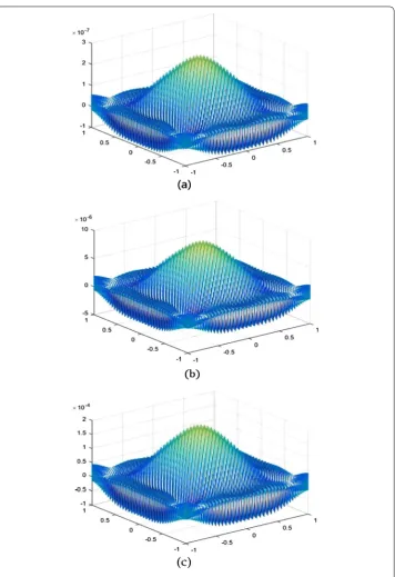
Photos (a), (b), and (c) in Fig. 5 show the errors between the analytical solutions and the CSM solutions whent= 0.3,t= 0.5, andt= 0.9, respectively, which indicate that the

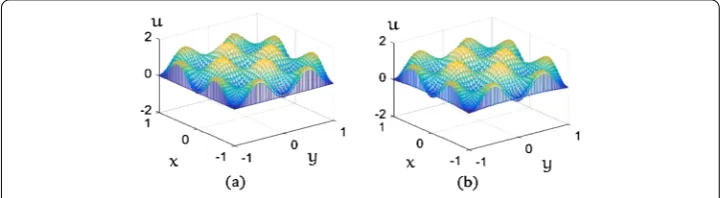
Figure 2(a) The analytical solution whent= 0.3. (b) The CSM solution whent= 0.3

Figure 3(a) The analytical solution whent= 0.5. (b) The CSM solution whent= 0.5

Figure 4(a) The analytical solution whent= 0.9. (b) The CSM solution whent= 0.9

numerical computational errors accord with the theoretical ones, because both errors are

O(10–4_{). This implies that the CSM scheme is very efficient and feasible for solving the 2D} Sobolev equations (1).

5 Conclusions and discussion

In this work, we have established the CSM scheme by means of the Chebyshev polyno-mials for the 2D Sobolev equations, analyzed the the existence, uniqueness, stability, and convergence of the CSM solutions. We have also used some numerical experiments to check the feasibility and effectiveness of the CSM scheme and to verity that the numerical computing results accord with the theoretical analysis ones. Moreover, it is shown that the CSM scheme is very valid and feasible for solving the 2D Sobolev equations.

Figure 5Errors between the analytical solutions and the CSM solutions: (a) att= 0.3, (b) att= 0.5, and (c) at

t= 0.9

Acknowledgements

The authors are thankful to the honorable reviewers and editors for their valuable suggestions and comments, which improved the paper.

Funding

This research was supported by the National Science Foundation of China grant 11671106.

Availability of data and materials

Competing interests

The authors declare that they have no competing interests.

Authors’ contributions

All authors contributed equally and significantly in writing this article. All authors wrote, read, and approved the final manuscript.

Author details

1_{School of Control and Computer Engineering, North China Electric Power University, Beijing, China.}2_{School of}

Mathematics and Physics, North China Electric Power University, Beijing, China.

Publisher’s Note

Springer Nature remains neutral with regard to jurisdictional claims in published maps and institutional affiliations.

Received: 30 January 2018 Accepted: 10 May 2018

References

1. Ting, T.W.: A cooling process according to two-temperature theory of heat conduction. J. Math. Anal. Appl.45(1), 23–31 (1974)

2. Shi, D.M.: On the initial boundary value problem of nonlinear equation of the migration of the moisture in soil. Acta Math. Appl. Sin.13(1), 31–38 (1990)

3. Liu, Y., Li, H., He, S., Gao, W., Mu, S.: A new mixed scheme based on variation of constants for Sobolev equation with nonlinear convection term. Appl. Math. J. Chin. Univ.28(2), 158–172 (2013)

4. Shi, D.Y., Wang, H.H.: Nonconforming H 1-Galerkin mixed FEM for Sobolev equations on anisotropic meshes. Acta Math. Appl. Sin.25(02), 335–344 (2009)

5. Guo, B.Y.: Spectral Methods and Their Applications. World Scientific, Singapore (1998)

6. Shen, J., Tang, T.: Spectral and High-Order Methods with Applications. Science Press, Beijing (2006)

7. Luo, Z.D., Jin, S.J.: A reduced-order extrapolation spectral-finite difference scheme based on the POD method for 2D second-order hyperbolic equations. Math. Model. Anal.22(5), 569–586 (2017)

8. An, J., Luo, Z.D., Li, H., Sun, P.: Reduced-order extrapolation spectral-finite difference scheme based on POD method and error estimation for three-dimensional parabolic equation. Front. Math. China10(5), 1025–1040 (2015) 9. Guo, B.Y.: Some progress in spectral methods. Sci. China Math.56(12), 2411–2438 (2013)

10. Jiang, Z.W., Chen, H.Z.: Error estimates for mixed finite element methods for Sobolev equation. Northeast. Math. J.

17(3), 301–314 (2001)

11. Gao, F.Z., Qiu, J.X., Zhang, Q.: Local discontinuous Galerkin finite element method and error estimates for one class of Sobolev equation. J. Sci. Comput.41, 436–460 (2009)

12. Shi, D.Y., Wang, H.H., Guo, C.: Anisotropic rectangular nonconforming finite element analysis for Sobolev equations. Appl. Math. Mech.29(9), 1203–1214 (2008)

13. Li, H., Luo, Z.D., An, J.: A fully discrete finite volume element formulation for Sobolev equation and numerical simulations. Math. Numer. Sin.34(2), 163–172 (2010)

14. Lu, W.J., Zhang, F.Y.: Long-time behavior of completely discrete Fourier spectral method of solutions to Sobolev equations. J. Natur. Sci. Heilongjiang Univ.18(2), 5–8 (2001)