Adaptive stabilized finite volume method and convergence analysis for the Oseen equations

R E S E A R C H

Open Access

Adaptive stabilized finite volume method

and convergence analysis for the Oseen

equations

Junxiang Lu

_{and Tong Zhang}

*_{Correspondence:} [email protected];

[email protected] 1_{School of Science, Xi’an}

Polytechnic University, Xi’an, China

2_{School of Mathematics &}

Information Science, Henan Polytechnic University, Jiaozuo, China

Abstract

In this paper, based on the pressure project method, we consider an adaptive stabilized finite volume method for the Oseen equations with the lowest equal order finite element pair. Firstly, we develop the discrete forms in both finite element and finite volume methods, and establish the existence and uniqueness of numerical solutions by establishing the equivalence of linear terms in finite element and finite volume methods. Secondly, a residual type a posteriori error estimator is designed, and the computable global upper and local lower bounds between the exact solutions and the finite volume solutions are established. Thirdly, a discrete local lower bound between two successive finite volume solutions is obtained, convergence analysis of the adaptive stabilized finite volume method is also performed. Finally, some numerical results are presented to verify the performances of the developed error estimators and confirm the established theoretical findings.

MSC: 65N15; 65N30; 76D05

Keywords: Adaptive algorithm; Stabilized finite volume method; Oseen equations; Convergence

1 Introduction

Finite volume method, as an important numerical tool for solving partial differential equa-tions, has been widely used in the engineering community for fluid computations (see [9,

14,15,29,30]). Finite volume method is intuitive since it is based on local conservation of mass, momentum, and energy over volumes. Finite volume method has a flexibility similar to that of the finite element method for handling complicated geometries, and its implementation is comparable to that of the finite difference method. Furthermore, its numerical solution usually has certain conservation features that are desirable in many practical applications. Based on the above reasons, several researchers have contributed to this method extensively and obtained numerous important results. For example, we can refer to [14,26] for the monographs, and for the recent developments about the finite volume method, we can read [1,8,13,20,31,37] and the references therein.

Let∈R2_{be a bounded polygon domain with Lipschitz continuous boundary∂. We} consider the following Oseen problem, which consists of finding a pair (u,p) as the solution

of the equations

⎧ ⎪ ⎪ ⎨ ⎪ ⎪ ⎩

–νu+ a· ∇u+∇p= f in,

∇ ·u= 0 in,

u= 0 on∂,

(1.1)

where u is the velocity field,pis the pressure,νis the viscosity, f is the body forces. For the sake of simplicity, we consider the simplest Dirichlet condition. Several simplifying as-sumptions will be made for the advection vector a. In particular, we take a∈C0_{(), weakly} divergence free with derivatives of order up tomis locally bounded (m> 0 is integer, see AssumptionA1in Sect.2).

The Oseen problem stated above can be considered as a linearization of the stationary incompressible Navier–Stokes equations. It also appears as one of the steps of some mul-tilevel methods for these equations, or results from a time discretization of the transient Navier–Stokes problem if the advection coefficient a is treated explicitly. This is why it is often used as a first step towards the analysis of the full nonlinear problem, to obtain both a priori and a posteriori estimates.

Let us introduce some standard notations. The space of square integrable functions in

is denoted byL2_{(), and the space of functions whose distributional derivatives of order} up tom≥0 belong toL2() is denoted byHm(). The spaceH₀1() consists of functions inH1_{() vanishing on∂. A bold character is used to denote the vector counterpart of} all these spaces. TheL2 _{inner product inis denoted by (·,·)}

, and the norm in a

Ba-nach spaceXby · X. This notation is simplified in some cases as follows: (·,·)≡(·,·),

· L2₍₎≡ · ₀, for the positive integerm, set · Hm₍₎≡ · m, and ifKis an element · L2_(K)≡ · K, · Hm_(K)≡ · m_,K.

With above notations, the velocity and pressure spaces for the continuous problem are

X:= H1₀(),M:=L2_{()/R. The variational formulation for problem (1.1) reads as follows:} For all (v,q)∈X×M, find (u,p)∈X×Msuch that

⎧ ⎨ ⎩

ν(∇u,∇v) – (∇ ·v,p) + (a·∇u, v) = (f, v), (∇·u,q) = 0.

(1.2)

The bilinear terms satisfy the following continuity and inf-sup properties (see [16]):

ν(∇u,∇v) – (∇ ·v,p) + (a·∇u, v) + (∇·u,q)

≤C∇u0+p0

∇v0+q0

, (1.3)

β∇u0+p0

≤ sup 0=(v,q)∈X×M

|ν(∇u,∇v) – (∇ ·v,p) + (a·∇u, v) + (∇·u,q)|

∇v0+q0

.

Here and below,C> 0 is a generic constant depending at most on the data,ν, a, and f. In the following sections,C1,C2, . . . denote some positive constants depending only on.

From the above properties, we know that problem (1.2) is well posed.

max{HK|K∈TH}. For simplicity, we assume that all the element domains are the image of a reference elementKthrough a polynomial mapping. We define the polynomial spaces

Pk(K) with orderk on the elementK. From these polynomial spaces, we construct the

finite element spacesXH⊂XandMH⊂Min the usual manner. The discrete version of

problem (1.2) is as follows: Find (uH,pH)∈XH×MHsuch that

⎧ ⎨ ⎩

ν(∇uH,∇vH) – (∇ ·vH,pH) + (a·∇uH, vH) = (f, vH), ∀vH∈XH,

(∇·uH,qH) = 0, ∀qH∈MH.

(1.4)

The well-posedness of problem (1.4) relies on the ellipticity of the viscous term and the inf-sup or the Babu˘ska–Brezzi condition (see [10,16]), which have been shown to hold for the continuous problem. The first property is automatically inherited by its discrete counterpart. However, the inf-sup condition needs to be explicitly required. This leads to the need to use mixed interpolations and verify

β∗≤ inf

0=qH∈MH_0=vsup_H∈XH

(∇ ·vH,qH) vH1· qH0

(1.5)

for a positive constantβ_∗. The construction of the finite element spacesXH andMHto

satisfy (1.5) can be found in [16], examples include the MINI element and the Taylor– Hood element.

From the computational point of view, it is convenient to use the same interpolation of the velocity and pressure. However, this choice turns out to violate condition (1.5); there-fore, some stabilized methods have been proposed to approximate problem (1.2). Exam-ples of these stabilized methods are those of Brezzi and Douglas [4], Brezzi and Pitkäanta [5], Douglas and Wang [12] (see also the references therein). Recently, a novel stabilized technique using polynomial pressure projection has been proposed and studied to solve incompressible flow [2,21,22,24]. This new stabilized method has three prominent fea-tures. (1) It is of practical convenience in real applications with the same partitions for velocity and pressure. (2) Less computational time is required by easily applying the lower order elements. (3) Compared with the standard finite element method, its analyses of

H1-norm andL2-norm for the velocity and pressure are derived without any high order regularity assumptions on the exact solution. So this method has been widely used to con-sider various kinds of problems [17,18,25,28,36].

In this paper, based on the regular triangularpartitionsof domainand the pressure project method, we consider the stabilized adaptive finite volume method for the Oseen equations by the lowest equal order element (i.e.,P1–P1pair). The main contributions of our work can be listed as follows.

(I) Existence and uniqueness of stabilized finite element and finite volume schemes are developed, the corresponding stability and convergence results can be established following the references [3,6,21].

(II) Residual type a posteriori error estimators are designed, the upper and lower bounds are presented, a discrete local lower bound between two successive numerical solutions is also shown.

The outline of this paper is organized as follows. In Sect.2, the stabilized finite element and finite volume methods for the Oseen problem are described. Our numerical schemes are based on the lowest equal order pair, and we use the polynomial pressure projection method to overcome the restriction of (1.5). The basic idea is to add some terms in the discrete schemes, which are formed by the local projection from different spaces. Hav-ing stated the stabilized numerical schemes, we deduce a complete numerical analysis of global upper and local lower bounds for the errors in Sect.3. Sections4and5are devoted to deriving the discrete local lower bound and the convergence property of the adaptive stabilized finite volume method. Two numerical examples are presented in Sect.6to show the performances of the developed error estimators. One with known solution to verify the convergence orders of the numerical solutions, the other is a model problem to con-firm the efficiency of the adaptive finite volume method. Finally, some conclusions are drawn.

2 Description of the discrete numerical schemes

2.1 Stabilized finite element method

Throughout this paper, we focus on the following finite element subspaces:

XH=

v∈C0()2∩X: v|K∈P1(K)2,∀K∈TH

,

MH=

q∈C0()∩M:q|K∈P1(K),∀K∈TH

,

whereP1(K) is the space of affine polynomials on the elementK.

For the solenoidal vector a, we make the following assumption (see [3,6,11]).

Assumption A1 There is a constantCDsuch that themderivatives of a within the

ele-mentKare bounded above byCD|a|∞,K,∀K∈Th.

Under the assumption of weakly divergence free of a, for all v∈X, we have

(a·∇v, v) =1 2

a·∇(v·v), 1= –1

2(∇·a, v·v) = 0. (2.1)

It is well known that the above chosen finite element spacesXHandMHdo not satisfy the

discrete inf-sup condition (1.5), but they are of practical importance in real applications. A recently popular stabilized approach, called local pressure projection method, is used in [2,17,21,22] to stabilize the lower order finite element for incompressible flow.

The stabilized finite element method for problem (1.2) is to find (uH,pH)∈XH×MH

satisfying

⎧ ⎨ ⎩

ν(∇uH,∇vH) – (∇ ·vH,pH) + (a·∇uH, vH) = (f, vH), ∀vH∈XH,

(∇·uH,qH) +Gh(pH,qH) = 0, ∀qH∈MH.

(2.2)

Here, the stabilized termG(·,·) is defined by

and the local projectionH:L2()→P0(K) satisfies

(p,qH) = (Hp,qH),Hp0≤Cp0, ∀p∈M,qH∈P0(K),

p–Hp0≤CHp1, ∀p∈H1()∩M,

(2.4)

whereP0(K) denotes a piecewise constant on each elementK.

We first present the Scott–Zhang [32] interpolating property as the following lemma.

Lemma 2.1 Let IHbe the interpolation operator from X∩C0()2into Xh.It holds w–IHw0,K≤C1HKw1,ωK,

w–IHw0,E≤C1HE1/2w1,ωE, IHw1≤ w1,

whereωK=

K∩K=∅K(K∈Th)andωE=

E∩K=∅K.

Due to the quasi-uniformness of the triangulationTH, the inverse inequality holds

wH1≤C2H–1wH0, ∀wH∈XH. (2.5)

Denote

B(uH,pH), (vH,qH)

≡ν(∇uH,∇vH) – (∇ ·vH,pH) + (a·∇uH, vH) + (∇·uH,qH) +Gh(pH,qH).

Then the well-posedness of problem (2.2) can be obtained from the following theorem.

Theorem 2.2 For all(uH,pH), (vH,qH)∈XH×MH,it holds

B(uH,pH), (vH,qH)

≤CuH1+pH0

vH1+qH0

. (2.6)

Furthermore,there exists a constantβ∗such that,for all(uH,pH)∈XH×MH,

β∗∇uH0+pH0

≤ sup 0=(vH,qH)∈XH×MH

|B((uH,pH), (vH,qH))| ∇vH0+qH0

. (2.7)

Proof The continuity (2.6) holds by using the Cauchy inequality and AssumptionA1. Now, we present the proof of (2.7). For eachpH∈MH⊂M, there exists w∈X[10,16]

such that

∇ ·w=pH (2.8)

and

Let wH=IHw∈XH, which satisfies Lemma2.1. Then it follows from the Green’s formula,

Poincare’s inequality, the inverse inequality (2.5), and (2.8)–(2.9) that

ν(∇uH,∇wH)≤νuH1wH1

≤νuH₁w₁≤C3νuH1pH0≤ 1 4pH

2

0+C23ν2uH21, (∇ ·wH,pH)= (∇ ·w,pH) –

∇ ·(w – wH),pH

≥ pH2₀–C1C4Hw1∇pH0 =pH2₀–C1C4Hw1

K∈TH

_∇(pH–HpH)₀

≥ pH2₀–C1C2C3C4pH0

K∈TH

pH–HpH0

≥3

4pH 2

0–C12C22C23C42pH–HpH20, (a·∇uH, wH)≤CD|a|∞∇uH0wH0

≤CD|a|∞∇uH0wH1≤ 1 4pH

2

0+C23CD|2 a|2∞uH21. Setδ> 0 and take

v_H= uH–δwH and qH=pH.

Thanks to (2.1) and the above inequalities, one finds

B(uH,pH), (uH–δwH,pH)

=ν(∇uH,∇uH) +Gh(pH,pH) + (a·∇uH, uH)

–δν(∇uH,∇wH) – (∇·wH,pH) + (a·∇uH, wH) ≥ν∇uH2₀+(I–H)pH2₀

–δC2₃ν2+C₃2C_D2|a|2_∞uH2₁–1 4pH

2

0+C12C22C23C42pH–HpH20

≥ν–δC2₃ν2+C₃2C2D|a|2_∞uH2₁+δ 4pH

2 0+

1 –δC2₁C₂2C₃2C₄2pH–HpH20,

provided that 0 <δ<min{ ν

C2

3(ν2+CD2|a|2∞),

1

C2

1C22C23C42}. Denote

C(ν)≡min

ν–δC₃2ν2+C2_D|a|2_∞,1 4δ

, C(δ)≡max2, 1 + 2δ2.

Then we have

∇vH2₀+qH2₀ =∇uH–δ∇wH20+pH20

≤2∇uH2₀+1 + 2δ2pH2₀≤C(δ)∇uH2₀+pH2₀.

Takingβ∗=C(ν)/C(δ), we obtain the desired result (2.7).

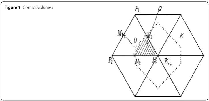
Figure 1Control volumes

2.2 Stabilized finite volume method

LetNHbe the set of all interior vertices of the triangulation andEHbe the set of all interior edges. To define the finite volume method, we introduce a dual partitionT_H∗ based on

TH, the elements inT_H∗are called control volumes. The dual mesh is constructed by the following rule: For each elementK∈THwith verticesPj,j= 1, 2, 3, select its barycenter

Oand the midpointMjon each of the edges ofK. We can construct the control volumes

Ki∈TH∗by connectingOtoMjas shown in Fig.1.

The dual finite element space is defined by

XH=

v∈L2()2: v|Ki∈P0(Ki)2, v|∂Ki∩∂= 0,∀Ki∈TH∗

.

Note thatP0(Ki) denotes a piecewise constant on each control volumeKi. The two finite

dimensional spacesXHandXHhave the same dimension. Furthermore, there exists an

invertible linear mappingH:XH→XHsuch that

HvH(x) =

NH

i=1

vH(xi)φi(x),xi is the node ofTH,x∈,vH∈XH,

whereφi(x) is the characteristic function associated with the dual partitionTH∗:

φi(x) =

⎧ ⎨ ⎩

1 x∈Ki,

0 otherwise.

The idea of connecting the different spaces through the mappingHwas introduced by

Li and Zhu in [27] for the elliptic problem. The following properties hold.

Lemma 2.3(See [7,26,34]) For anyvH∈XHandv∗H=HvH∈XH,for each interior

ele-ment K∈THwith its boundary∂K∈EH,there hold

K

vH– v∗H

dx= 0,

∂K

vH– v∗H

ds= 0, v∗_H0≤CvH0, vH– v∗H0,r,K≤ChKvH1,r,K, vH– v

∗

H0,r,∂K≤CH

1–1/r

Analogous to (2.2), the stabilized finite volume method for problem (1.1) is to find (uv

H,pvH)∈(XH,MH) satisfying

⎧ ⎨ ⎩

A(uv_H,HvH) +D(HvH,pvH) + (a·∇uvH,HvH) = (f,hvH), ∀vH∈XH,

(∇ ·uv

H,qH) +GH(pvH,qH) = 0, ∀qH∈MH,

(2.10)

where

Auv_H,hvH

= –ν

NH

j=1

v_H(Pj)·

∂Kj ∂uv

H ∂n ds,

DHvH,pvH

=

NH

j=1

vH(Pj)·

∂Kj

pv_H·nds,

(f,HvH) =

NH

j=1

vH(Pj)·

Kj

fdx.

Lemma 2.4 It holds that,for alluv_H, vH∈XH,pvH∈MH,

Auv_H,HvH

=ν∇uv_H,∇vH

,

DHvH,pvH

=∇ ·vH,pvH

.

(2.11)

Moreover,we have

a·∇uv_H,uv_H= 0. (2.12)

Proof The equations in (2.11) have been shown in [23,34,35]. It suffices to prove (2.12). For uv

H∈XH, it follows from the definition ofhand (2.1) that

a·∇uv_H,uv_H=

NH j=1 Kj

a·∇uv_H·HuvHdx

= –

NH

j=1

HuvH(Pj)·

Kj

a·∇uv_Hdx

=

NH

j=1

HuvH(Pj)·

Kj

(∇ ·u)uv_Hdx–

∂Kj

auv_H·nds

.

With the weakly divergence free of a and the continuity of a, uv

H, we complete the

proof.

We denote the generalized bilinear formC((·,·), (·,·)) on (XH,MH)×(XH,MH) as

Cuv_H,pv_H, (vH,qH)

=Auv_H,HvH

+DHvH,pvH

+duv_H,qH

+GH

pv_H,qH

+a·∇uv_H,HvH

By applying the relationships between finite element and finite volume methods pre-sented in Lemma2.4, and following the proof of Theorem2.2, we can establish the conti-nuity and weak coercivity for the generalized bilinear formC((·,·), (·,·)). Here we omit the proof for simplification and present its continuity and weak coercivity.

Theorem 2.5 For all(uv_H,pv_H), (vH,qH)∈XH×MH,it holds

Cuv_H,pv_H, (vH,qH)≤CuvH1+p

v H0

vH1+qH0

.

Moreover,there exists a constantβ∗> 0,independent of H,such that

β∗uv_H

1+p

v H0

≤ sup 0=(vH,qH)∈(XH,MH)

C((uv

H,pvH), (vH,qH)) vH1+qH0

. (2.13)

From Theorem2.5, we know that problem (2.10) has a unique solution (uv_H,pv_H). For the stability and convergence results of numerical schemes (2.2) and (2.10), following the proofs provided in [3,6,21], by taking different test functions and using the energy method, we can obtain that the numerical schemes (2.2) and (2.10) are unconditionally stable, error estimates for the numerical solutionsare also optimal. Here we omit these proofs for simplification.

3 A posteriori error estimation

In this section, we derive a residual type error estimator of the stabilized finite volume method for the Oseen problem. The upper and lower bounds between the exact solution and the finite volume solution are obtained by using Lemma2.4and some techniques involving the bubble functions.

3.1 Upper bounds

In this subsection, a residual-based error estimator is investigated by using the techniques of residual a posteriori error estimates and the stabilized finite volume method for the Oseen equations. The error between (u,p) and (uv

H,pvH) is bounded by the global error

estimatorηHdefined below.

For an elementKof the triangulationTH, we set

RK= f +νuvH–∇pvH– a·∇uvH,

and for an edgeEof a triangleK

JE=

ν∂u v H ∂n –p

v HI·n

E

=

ν∂u v H ∂n

E

,

where n is the unit normal outward to∂K. We also define the following local error esti-mator for any (uv_H,pv_H)∈XH×MH:

η2_H(K) =H_K2RK2_0,K+∇ ·uv_H2

0,K+HEJE

2 0,E.

Then the global error estimator is given by

η2_H=

The following theorem plays an important role in the process of establishing the upper bound of adaptive finite volume method for the Oseen equations.

Theorem 3.1 Let(u,p)and(uv_H,pv_H)be the solutions of problems(1.2)and(2.10), respec-tively.Then,for any(v,q)∈X×M andv∗_H∈XH,it holds

ν∇u– uv_H,∇v–∇ ·v,p–pv_H+∇ ·u– uv_H,q+a· ∇u– uv_H, v

=

K∈TH

K

RK·

v– v_H∗+∇ ·uv_Hqdx+

E∈EH

E

JE

v– v∗_Hds. (3.1)

Proof It follows from (1.2) that

ν∇u– uv_H,∇v–∇ ·v,p–pv_H+∇ ·u– uv_H,q

= (f, v) – (a·∇u, v) –ν∇uv_H,∇v+∇ ·v,pv_H–∇ ·uv_H,q. (3.2) By the Green’s formula, one finds

ν∇uv_H,∇v–∇ ·v,pv_H+∇ ·uv_H,q

=–νuv_H+∇pv_H, v+∇ ·uv_H,q+

E∈EH

E

JE·vds. (3.3)

On each control volumeK∈T_H∗, applying the Green’s formula onK∩K(see Fig.1), we have

K∩K

–νuv_H+∇pv_H·v∗_Hdx= –

∂K∩K

JE·v∗Hds–

∂K∩K

JE·v∗Hds.

Summing the above results and using the first equation in (2.10), we obtain

0 =–νuv_H+∇pv_H, v∗_H+f, v∗_H–a·∇uv_H, v∗_H+

E∈EH

E

JE·v∗Hds

=–νuv_H+∇pv_H, v∗_H+f, v∗_H+a·∇uv_H, u – v_H∗

+

E∈EH

E

JE·v∗Hds–

a·∇uv_H, v. (3.4)

The proof is completed by using (3.2), (3.3), and (3.4).

Theorem 3.2 Let(u,p)and(uv_H,pv_H)be the solutions of problems(1.2)and(2.10), respec-tively.Under AssumptionA1,there exists a positive constant C such that

_∇

u– uv_H0+p–pv_H0≤C5ηH.

Proof Using Lemmas2.1and2.3and the Cauchy–Schwarz inequality in (3.1), we see that

K∈TH

K

RK·(v –IHv)dx

≤C1

K∈Th

H_K2RK2_0,K

1/2

K∈TH

K∇ ·

uv_H·q dx≤

K∈TH

_{∇ ·}uv_H0,K· q0,

E∈EH

E

JE·(v –IHv)ds

≤C1

E∈Eh

HEJE2_0,E

1/2

v1.

It follows from the above inequalities, Lemma2.3, and the coerciveness property (1.3) that

β∇u– uv_H0+p–pv_H0

≤ sup 0=(v,q)∈X×M

ν∇u– uv_H,∇v–∇ ·v,p–pv_H+a· ∇u– uv_H, v

+∇ ·u– uv_H,q/∇v0+q0

≤C5

K∈TH

H_K2RK2K+

K∈TH

_{∇ ·}uv_H2_K+

E∈EH

HEJE2_E

1/2

≤C5ηH.

Thus, we complete the proof.

3.2 Lower bounds

This subsection is devoted to estimating the lower bound of the residual based error esti-mator. Here, it is important to ensure the efficiency of an algorithm that usesηHas a local

refinement indicator. Firstly, we recall the definition of the oscillation of the residual on each elementK∈TH:

OSC_R2(K)≡HK(RK–RK)

2

K, OSC

2

D(K) =∇ ·uvH

2

K,

where RK is defined byRK =_|K1_|

KR dx,|K|is the area of an elementK. Moreover, we

define the oscillation of the jump on each edgeEby

OSC_J2(E)≡HEJE–JE2E=HE

∂uvH

∂n – 1

HE

E ∂uv_H

∂n ds

2

E

= 0.

Then the local oscillation is defined by

OSCH(K) =

OSC2_R(K) +OSC2_D(K) +OSC_J2(E)1/2

and the global oscillation by

OSCH= K∈TH

OSC_R2(K) +OSC_D2(K) 1 2

=

K∈TH

_HK(RK–RK)2

K+∇ ·u v H 2 K 1 2 .

coordi-nates ofK. Define the triangular bubble function bKby

bK(K) =

⎧ ⎨ ⎩

27λK,1λK,2λK,3, inK,

0, in\T. (3.5)

Also, for anyE∈EH, let the barycentric coordinates of the end points ofEbeλE,1andλE,2, and define the edge bubble functionbEby

bE(K) =

⎧ ⎨ ⎩

4λE,1λE,2, inωE,

0, in\ωE,

(3.6)

whereωEis defined in Lemma2.1. The following results can be found in reference [33].

Lemma 3.3 Assume that the partitionTHis locally quasi-uniform.For any element K∈TH and edge E∈EH,the functionsbKand bEsatisfy the following properties:

(1) suppbK⊂K,bK∈[0, 1],andmaxx∈KbK(x) = 1;

K bKdx=

9

20|K| ∼H 2

K, ∇bK0,K≤CHK–1bKK.

(2) suppbE⊂ωE,bE∈[0, 1],andmaxx∈ωEbE(x) = 1;

E

bEdx=

2 3HE,

ωE

bEdx∼HE2, ∇bEωE≤CH

–1

E bEωE. Lemma 3.4 For any K∈THand(uv

H,pvH)∈XH×MH,under AssumptionA1,we have HKRKK≤C∇

u– uv_HK+p–pv_HK+HK(RK–RK)_K

, (3.7)

H

1 2

EJE_E≤C∇

u– uv_Hω

E+p–p v

HωE+HK(RK–RK)ωK

. (3.8)

Proof It follows from (1.2), (2.1), inverse inequality, the Green’s formula, and Lemma3.3

that

R1K2K =

20 9

K

bKR1KRKdx+

K

bKRK(RK–RK)dx

K

≈f+νuv_H– a·∇uv_H–∇pv_H, bKRK

K+

K

bKRK(RK–RK)dx

=ν∇u,∇(bKRK)

K–

p,∇ ·(bKRK)

K+ (a· ∇u, bKRK)K

–ν∇uv_H,∇(bKRK)

K

+pv_H,∇ ·(bKRK)

K–

a·∇uv_H, bKRK

K+

K

bKRK(RK–RK)dx ≤CH_K–1∇u– uv_HK+p–pv_HK+RK–RKK

RKK.

Thus we have

R1KK≤C

H_K–1∇u– uv_HK+p–pv_HK+RK–RKK

Thanks to the triangle inequality, one finds

HKRKK≤ HKRKK+HK(RK–RK)_K

≤C∇u– uv_HK+p–pvHK+HK(RK–RKK)

.

That is, the proof of (3.7) is completed.

Similar to the proof of (3.7), using (1.2), Lemmas2.1and3.3and noting [23,37], we obtain

_Eν∇u– uv_H· ∇(bEJE)dx–

E

p–pv_H· ∇ ·(bEJE)dx

≤CH_E–1/2∇u– uv_Hω

E+p–p v HωE

JEE,

E

bEJE(JE–JE)ds

≤CJE–JEEbEJEE= 0,

_Ef +νuv_H– a·∇uv_H–∇pv_H·bEJEdx+

E

a·∇u– uv_H·bEJEdx

≤CH_E1/2RKωE+H

1/2

E CD|a|∞∇

u– uv_Hω

E

JEE.

Thus we have

JE2_E=3 2

E

JEbEJEds+

E

bEJE(JE–JE)ds

≈

E

–νuv_H+∇p_Hv·bEJEdx–

E

ν∇uv_H–pv_H· ∇(bEJE)dx+

E

bEJE(JE–JE)ds ≤

E

ν∇u– uv_H· ∇(bEJE)dx–

E

p–pv_H· ∇ ·(bEJE)dx+

E

bEJE(JE–JE)ds

–

E

f+νuv_H– a·∇uv_H–∇pv_H·bEJEdx+

E

a· ∇u– uv_H·bEJEdx

≤CH_E–1/2∇u– uv_Hω

E+p–p v HωE

+H_E1/2RKωE

JEE. (3.9)

Then (3.8) is obtained by the triangle inequality, (3.7), and (3.9).

Using Lemma3.4and taking a sum over all elements and edges, we obtain the following result.

Theorem 3.5 Let(u,p)∈X×M and(uv

H,pvH)∈XH×MHbe the solutions of problems

(1.2)and(2.10),respectively,then we have

ηH≤C∇

u– uv_H0+p–pv_H0+OSCH

.

4 Discrete local lower bound

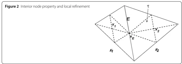
Figure 2Interior node property and local refinement

EofTH(see [37]): The interior ofE=∂K1∩∂K2(K1,K2∈TH) contains at least one vertex ofTH, see Fig.2.

Compared with the results of the residual-based error estimator in the previous section, we focus on the discrete local lower bound on the domainωEfor eachE∈EH.

Lemma 4.1 Under the assumption of the interior node property,let(uv

h,pvh)∈Xh×Mhand

(uv

H,pvH)∈XH×MHbe the stabilized finite volume solutions of problem(2.10)onThand TH,respectively.Then,for Ki∈ωE(i= 1, 2),we have

HKiRKi0,Ki≤C∇

uv_h– uv_H0,Ki+p_hv–pv_H0,Ki+OSCH(K)

.

Proof The triangle inequality gives

RKi0,Ki≤ RKi–RKi0,Ki+RKi0,Ki. (4.1)

For the second term on the right-hand side of (4.1), choosing vi=IHbKi, v∗i =Hvi∈XH∗

and applying Lemmas2.4and3.3, the inverse inequality, and the interior node property, we see that

RKi2_0,Ki∼RKi, v∗iRKi

=f +νuv_H– a·∇uv_H–∇pv_H, v∗_iRKi

–RKi–RKi, v∗iRKi

=Auv_h– uv_H, v∗_iRKi

+Dpv_h–pv_H, v∗_iRKi

+a· ∇uv_h– uv_H, v∗_iRKi

–RKi–RKi, v∗iRKi

=ν∇uv_h– uv_H,∇(IHbKiRKi)

+∇ ·(IHbKiRKi),p

v h–pvH

+a· ∇uv_h– uv_H, v∗_iRKi

–RKi–RKi, v∗iRKi

≤CH_Ki–1∇uv_h– uv

H0,Ki+p v

h–pvH0,Ki

+CD|a|∞∇

uv_h– uv

H0,Ki+RKi–RKi0,Ki

RKi0,Ki.

Therefore, thanks to (4.1) we have

RKi0,Ki≤C

H_Ki–1∇uv_h– uv_H0,Ki+pv_h–pv_H0,Ki+RKi–RKi0,Ki

.

Multiplying the above inequality byHKi, a straightforward computation gives the desired

Lemma 4.2 Under the assumption of the interior node property,let(uv_h,pv_h)∈Xh×Mhand

(uv

H,pvH)∈XH×MHbe the stabilized finite volume solutions of problem(2.10)onThand TH,respectively.Then,for E∈EH,we have

H_E1/2JE_0,E≤C∇

uv_h– uv_H0,Ki+p_hv–pv_H0,Ki+OSCH(K)

.

Proof Setting vE=IHbEand vE∗=HvEand noting that [pvHI·n]E= 0, we have

JE2_0,E∼JE, v∗EJE

=

ν∂u v H ∂n –p

v

HI·n, vE∗JE

. (4.2)

Using the Green’s formula and the divergence theorem on eachQ∈K∩K, we get (see Fig.1)

ν∂u v H ∂n , v

∗ E E = –

∂Ki ν∂u

v H ∂n ·v

∗

Eds+

Q

νuv_H·v∗_Edx,

pv_HI·n, v∗_EE= –

∂Ki

pv_H·nv∗_Eds+

Q

∇pv_H·v_E∗dx.

Using the above equalities and recalling the definitions ofA(·,·) andD(·,·), we see that

ν∂u v H ∂n –p

v HI·n, v∗E

E

= –

∂Ki

ν∂u v H ∂n –p

v HI·n

·v∗_Eds+

Q

νuv_H–∇pv_H·v∗_Edx

=

Q

f– a· ∇uv_H+νuv_H–∇pv_H·v∗_Edx.

Due tosuppbE⊂ωE, multiplyingJEto both sides of the above equality, we obtain

Q

f– a· ∇uv_H+νuv_H–∇pv_H·JEvE∗dx

≤CRK0,ωEJEv

∗

E0,ωE≤CH

1/2

E RK0,ωEJE0,ωE. (4.3)

Combine (4.2) with (4.3) to arrive at

H_E1/2JE_0,E≤CHKiRK0,ωE. (4.4)

The proof is completed by using Lemma4.1and (4.4).

Finally, from Lemmas4.1and4.2, we obtain the main result of this section.

Theorem 4.3 Under the assumption of the interior node property,let(uv_h,pv_h)∈Xh×Mh

and(uv

H,pvH)∈XH×MHbe the stabilized finite volume solutions of problem(2.10)onTh

andTH,respectively.Then we have

ηH≤C6∇

uv_h– uv_H0+pv_h–pv_H0+OSCH

5 Adaptive finite volume method and convergence analysis

In this section, we develop an adaptive finite volume method based on the local error estimator presented in the previous sections. The techniques are adopted from [23,37] for the second order elliptic problem. For the Oseen equations, the adaptive finite vol-ume method can be divided into several steps. For the sake of convenience, we setTk,

k= 0, 1, 2, . . . , to be a sequence of shape regular triangulations and (uv

k,pvk),k= 0, 1, 2, . . . ,

to be a sequence of stabilized finite volume solutions on the corresponding nested finite element spaces generated by the adaptive finite volume method. We have developed the quasi-residual type of the a posteriori error estimator and established the upper and lower bounds between the exact solution and the finite volume solutions, and the discrete local lower bounds between the approximate solutions on meshesTHandThin Sects.3and4.

5.1 Adaptive finite volume method

First, we choose parametersθ1,θ2∈(0, 1) and an initial meshT0with mesh sizeh0=H.

Step1. Solve and estimate.

1. Solve the following stabilized finite volume formulation to find(uv k,pvk):

Cuv_k,pv_k, (vk,qk)

=f,v∗_k.

2. Compute the residual error estimatorηhk.

Step2. Local refinement.

1. Determine a suitable adaptive refinement for an update. LetUkbe the minimal edge set required refinement by satisfying the following marking strategy:

θ1ηhk≤ηhk(ωUk), θ2OSChk≤OSChk(ωUk).

2. Refinement and completion. LetTk+1be the refinement ofTk. Refine each element

K∈ω_Ukand complete the hanging points, such thatTk+1is a conforming triangulation.

Step3. Cycle criterion: For a sufficiently small toleranceε> 0, ifηhk≤ε, stop the

com-putation. Otherwise, setk=k+ 1 and go to Step 2.

The convergence analysis for the adaptive stabilized finite volume method will be dis-cussed in what follows. It is known that the convergence analysis of finite element method requires the orthogonality property [23,37]. However, the corresponding property loses effectiveness for the finite volume method due to the test and trial functions that belong to different spaces for the present method.

Theorem 5.1 Set (uv_h,pv_h)∈Xh ×Mh and(uvH,pvH)∈XH×MH be the stabilized finite

volume solutions of problem(2.10)onTh andTH,respectively.Denote eh = uvh– uvH and h=pvh–pvH.Then we have

ν∇u– uv_H,∇eh

–∇ ·eh,p–pvH

+∇ ·u– uv_H,h

+a· ∇u– uv_H,eh

≤C∇uv_h– uv_H0+pv_h–pv_H0·OSCH.

Proof Choosing (v,q) = (vH,qH) in (3.1), it follows from Lemma2.3and Theorem3.1that

K

RK·

vH– v∗H

dx=

K

(RK–RK)·

vH– v∗H

_K∇ ·uv_HqHdx

≤∇ ·uv_H

0,KqH0,K, ∀K∈TH,

_EJE

v– v∗_Hds=

E

(JE–JE)

v– v∗_Hds= 0, ∀E∈∂K.

Summing up over allK∈THandE∈EHwith (vH,qH) = (eh,h) and using the definition of

OSCH, we obtain the desired result.

5.2 Error reduction of two successive steps

The convergence property guarantees that the iterative loop terminates in a finite number of steps starting from an initial coarse mesh. Now, we investigate the adaptive stabilized finite volume method for the Oseen equations in terms of an error reduction between two successive steps. The mathematical induction argument can be used to obtain the error reduction in a finite number of steps.

Lemma 5.2 Let(uv

h,pvh)∈Xh×Mhand(uvH,pvH)∈XH×MHbe the stabilized finite volume

solutions of problem(2.10)onTh andTH,respectively.Set H=maxK∈THHK.Then there

exists a constantρ1∈(0, 1)such that

OSC_h2≤ρ1OSCH2.

Proof Here, we only estimate the termRτ,τ∈Th(see Fig.2). Others can be bounded with a similar argument. For the residual onτ⊂K⊂TH, we have

Rτ =RHτ –∇

∇pv_h–∇pv_H– a·∇uv_h–∇uv_H, (5.1)

whereRτandRHτ are the error estimators on meshThwith solutions (uvh,pvh) and (uvH,pvH),

respectively. Using the definition ofRτ, (5.1) and the Young inequality, we see that

OSC_h2(K) = τ⊂K

h2_τRτ–Rτ20,τ+

τ⊂K

_{∇ ·}uv_h2_0,τ. (5.2)

Since∇h=∇(pv_h–pHv) is a constant, thus∇h–∇h= 0. Settingγ0∈(0, 1) such that

hτ ≤γ0HKandK∈ωUH, we define a refinement factor by

γK=

⎧ ⎨ ⎩

γ0, inK∈ωUH,

1, in\ω_UH.

Thanks to (2.4), (5.2), the making strategy on local refinement and straightforward com-putation, the above inequality restricted to the meshTHcan be rewritten as

OSC_h2 =

K∈TH

τ⊂K

OSC2_h(τ)

≤ K∈TH

γ_K2H_K2Rτ –Rτ2_0,K+

K∈TH

_{∇ ·}uv_h2_0,K

≤

K∈TH\ωUK γ₀2

H_K2Rτ–Rτ2_0,K+

K∈TH

_{∇ ·}uv_h2_0,K

+

K∈ω_U

K γ₀2

H_K2Rτ–Rτ20,K+

K∈TH

_{∇ ·}uv_h2

0,K

+1 –γ₀2 K∈TH

_{∇ ·}uv_h2

0,K

≤2OSC_H2 –1 –γ₀2 K∈UK

OSC2_H(τ)

≤2 –1 –γ₀2θ₂2OSC_H2.

Thus, the desired result is obtained by choosingρ1= 2 – (1 –γ02)θ22∈(0, 1) in the above

inequality.

Lemma 5.3 Let(uv

h,pvh)∈Xh×Mhand(uvH,pvH)∈XH×MHbe the stabilized finite volume

solutions of problem(2.10)onTh andTH, respectively.There exist constants γ > 0and

ρ0∈(0, 1)such that

u– uv_h1+p–pv_h0+γOSC_h2≤ρ0u– uvH1+p–p

v

H0+γOSC 2

H

.

Proof Using (1.3) and the Young inequality, we have u– uv_h2₁+p–pv_h2₀

=u– uv_H2₁–uv_h– uv_H12– 2∇u– uv_h,∇uv_h– uv_H

+p–pv_H02–pv_h–pv_H2₀– 2p–pv_h,pv_h–pv_H

≤u– uv_H2₁+p–pv_H2₀–uv_h– uv_H2₁+pv_h–pv_H2₀

+ 2u– uv_h1+p–pv_h0·uv_h– uv_H1+pv_h–pv_H0

≤u– uv_H2₁+p–pv_H2₀–uv_h– uv_H2₁+pv_h–pv_H2₀

+β–1ν∇u– uv_h,∇uv_h– uv_H–∇ ·uv_h– uv_H,p–pv_h

+a· ∇u– uv_h, uv_h– uv_H+∇ ·u– uv_h,pv_h–pv_H. (5.3)

By Theorem5.1and the Young inequality, we obtain

β–1ν∇u– uv_h,∇uv_h– u_Hv–∇ ·uv_h– uv_H,p–pv_h

+a· ∇u– u_hv, uv_h– uv_H+∇ ·u– uv_h,pv_h–pv_H

≤C7uvh– uvH1+p

v h–pvH0

·OSCh ≤1

2u

v h– uvH

2 1+p

v h–pvH

2 0

+C₇2OSC_h2. (5.4)

Combine (5.3) with (5.4) and apply Lemma5.2to arrive at

u– uv_h2₁+p–pv_h2₀+γOSC_h2

≤u– uv_H2₁+p–pv_H2₀–1 2u

v h– uvH

2 1+p

v h–pvH

2 0

whereC8= (ρ1C72+γρ1). By the results of a lower bound of the solution on the initial mesh and Theorems3.2and4.3, and the marking strategy, we have

u– uv_H2₁+p–pv_H2₀≤C₅2η_H2 ≤C₅2θ₁–2η2_H(ω_Uk)

≤C9uvh– uvH

2 1+p

v h–pvH

2 0+OSC

2

H

, (5.6)

whereC9= 2C25C62θ1–2. Substituting (5.6) into (5.5), we see that u– uv_h2₁+p–pv_h2₀+γOSC_h2

≤

1 – 1

2C9

u– uv_H2₁+p–pv_H2₀+

C8+ 1 2

OSC_H2.

Choose appropriate parametersθ1> 0 andγ> 0 such that

1 – 1 2C9

= 1 – θ 2 1

2C₅2C2₆ ∈(0, 1) and C8+

1 2=ρ1C

2 7+γρ1+

1 2∈(0, 1).

Settingρ0=max{1 –_2C1₉,C8+1₂}, we complete the proof. Using induction for a series of partitionsTk,k= 0, 1, 2, . . . , we obtain the convergence of adaptive stabilized finite volume method.

Theorem 5.4(Convergence analysis) Let(uv

k,pvk),k= 0, 1, 2, . . . ,be a sequence of the

cor-responding stabilized finite volume solutions of problem(2.10)onTk,set the mesh size H of

T0be sufficiently small.Then we have

u– uv_h1+p–pv_h0≤u– u_Hv₁+p–pv_H0+γOSC_H21/2ρ₀k.

From Theorem5.4, we can see that our algorithm will terminate in a finite number of steps.

6 Numerical validations

In this section, we present two numerical examples to confirm our theoretical results and verify the efficiency of established a posteriori error estimators for the Oseen equations in the stabilized finite volume method. We solve the considered problem in the following adaptive strategy as presented in Sect.5.

(1) Give an initial triangulationThand a toleranceη∗. Solve the Oseen equations by the stabilized finite volume method on this partition.

(2) If{_K∈T

hη

2

K}1/2_≤η∗_{, stop, we get the final numerical approximations. Otherwise,}

go to (3).

Table 1 Errors and the effective index on adaptive meshes withν= 1

N ratio uh_u–₁u1 u_H1rate ph_p–₀p0 p_L2rate

550 0.5437 0.372325 0.875961

851 0.5404 0.323236 0.6478 0.737632 0.7875 1234 0.5650 0.262181 1.1267 0.610745 1.0159 1865 0.6187 0.217119 0.9133 0.501487 0.9545 3011 0.6869 0.174988 0.9007 0.394036 1.0068

Table 2 Error and the effective index on uniform meshes withν= 1

N ratio uh_u–₁u1 u_H1rate ph_p–₀p0 pL2rate

550 0.5437 0.372325 0.875961

857 0.5557 0.356411 0.1970 0.827581 0.2562 1241 0.5491 0.340932 0.2399 0.796662 0.2057 1872 0.5532 0.332744 0.1183 0.752626 0.2766 3032 0.5721 0.309528 0.3001 0.703231 0.2815

(3) ComputeηKand{

K∈Thη

2

K}1/2, generate the new mesh sizeh, and re-compute {K∈Thη

2

K}1/2based on the new partition, then go to step (2).

6.1 A singular problem with known solution

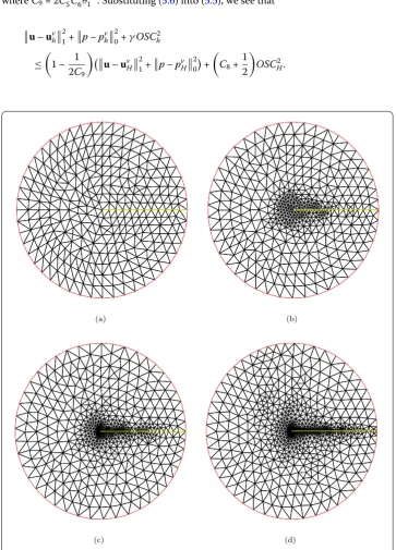
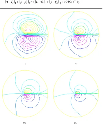
In this test, we compute the Oseen equations inwith adaptive mesh and uniform mesh, whereis a disk of radius equal to 1 with a crack joining the center to the boundary as presented in [33], and the exact solutions for velocity and pressure are given by

u1= 1.5r 1

2_{cos(0.5θ) –cos(1.5θ),}

u2= 1.5r 1

2_{3sin(0.5θ) –sin(1.5θ),}

p= –6r–12_cos(0.5θ),

where (r,θ) is a polar representation of a point in the disk and these solutions are singular at the end of the crack.f is determined by (1.1), and non-homogeneous Dirichlet bound-ary conditions on the curved part of the boundbound-ary and homogeneous Dirichlet boundbound-ary conditions on the straight part of the boundary are given. We choose the advection

cient a =1₁andν= 1. We start our adaptive computation from the initial triangulations, as presented in Fig.3(a) and refine three times shown in Fig.3(b)–(d). It is observed that there are much more elements in the noncontinuous area than in the continuous area. Furthermore, the contours of the pressure near the crack become smooth as the num-ber of triangles increases, see Fig.4(a)–(d). In Tables1–2, we provide the ratio between the error indicators and the discrete error, which is defined as the effective index in [19]. For a good estimator, this quantity should be a constant, independent of the mesh sizes. HereNT is the number of elements in the triangulations. The relative errors of veloc-ity and pressure in different norms are presented in adaptive mesh and uniform mesh. The experimental convergence rates are given byαeθ =

2∗log[eθ(ε1)0/eθ(ε2)0]

log[NT(ε1)/NT(ε1)] , whereθtakes

u,p.

Comparing Tables1and2, we can see that the error estimator is good due to the ra-tio being a constant near 0.55. Since the convergence order of the relative errors of ve-locity and pressure are O(h), then we can conclude that the convergence order of er-ror estimator is O(h), which verifies the established theoretical analysis very well. On the other hand, the errors of adaptive procedures decrease much faster than those ob-tained by uniform ones. For example, the precision obob-tained with 3032 triangles in a

uniform mesh can be reached with 1234 triangles in an adaptive computation. This means we can save more work by the adaptive procedures than by the uniform proce-dures.

6.2 T-shape domain model

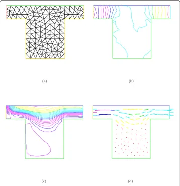
A T-shape domain model, as shown in Fig.5, is a popular problem for testing the efficiency of the established a posteriori error estimators. In this test, we chooseu= (4y(1 –y), 0) on influx and natural boundary condition on outflux.

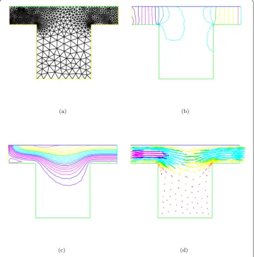
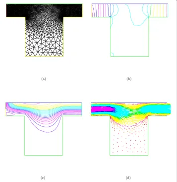
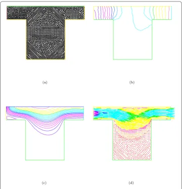
We start from the initial mesh withh= 0.25, the corresponding profiles of velocity and pressure are presented in Fig.6. Then we note that the successive iterations of the adap-tive strategies create more triangles in two corners of the T-shape domain as time in-creases, see Figs.7–8. The profiles of velocity and pressure level lines are also presented with adaptive computations, see Figs.7–8. As expected, the oscillations in the obtained pressure isovalues disappear and the velocity field becomes smooth. Finally, in order to show the prominent features of the established a posteriori error estimators, we com-pare the velocity and pressure contours obtained in the adaptive mesh with the uniform mesh using nearly the same number of triangles, see Figs.8and9. From these figures, we

Figure 9The mesh, the profiles of pressure and velocity, and the velocity vector with NT = 2876

can see that the obtained results using the adaptive algorithm based on the a posteriori error estimators give more accurate approximation to the exact solutions in the critical regions.

7 Conclusion

Acknowledgements

JXL and TZ express their gratitude to Shoujin Li for his discussions on this paper.

Funding

This work is supported by the National Natural Science Foundation of China (Nos. 11601410, 11601411), Shaanxi Natural Science Foundation (No. 2017JM1007), the Foundation for University Key Teacher by the Henan Province (2016GGJS-045), and the FDYS of Henan Polytechnic University (J2015-05).

Abbreviations

Not applicable.

Availability of data and materials

Not applicable.

Ethics approval and consent to participate

JXL gave some comments on the writing and revision of the paper, JXL also took part in the proof of error reduction. TZ wrote and revised the paper. They have no competing interests.

Competing interests

JXL and TZ declare that they have no competing interests.

Consent for publication

JXL and TZ read and approved the final version of the manuscript.

Authors’ contributions

JXL presented some comments on the writing and revising of the paper and took part in the proof of error reduction. TZ wrote and revised the paper. Both authors read and approved the final manuscript.

Publisher’s Note

Springer Nature remains neutral with regard to jurisdictional claims in published maps and institutional affiliations.

Received: 8 March 2018 Accepted: 31 July 2018

References

1. Bi, C.J., Wang, C.: A posteriori error estimates of finite volume element method for second order quasilinear elliptic problems. Int. J. Numer. Anal. Model.13(1), 22–40 (2016)

2. Bochev, P., Dohrmann, C., Gunzburger, M.: Stabilization of low-order mixed finite elements for the Stokes equations. SIAM J. Numer. Anal.44, 82–101 (2006)

3. Braack, M., Burman, E., John, V., Lube, G.: Stabilized finite element methods for the generalized Oseen problem. Comput. Methods Appl. Mech. Eng.196, 853–866 (2007)

4. Brezzi, F., Douglas, J.: Stabilized mixed methods for the Stokes problem. Numer. Math.53, 225–235 (1988) 5. Brezzi, F., Pitkäanta, J.: On the stabilization of finite element approximation of the Stokes problem. In: Hackbush, W.

(ed.) Efficient Solution of Elliptic Systems, pp. 11–19. Vieweg, Braunschweig (1984)

6. Burman, E., Fernandez, M.A., Hansbo, T.: Continuous interior penalty finite element method for Oseen’s equations. SIAM J. Numer. Anal.44, 1248–1274 (2006)

7. Chatzipantelidis, P., Makridakis, C., Plexousakis, M.: A-posteriori error estimates for a finite volume method for the Stokes problem in two dimensions. Appl. Numer. Math.46, 45–58 (2003)

8. Chen, C.J., Zhao, X.: A posteriori error estimate for finite volume element method of the parabolic equations. Numer. Methods Partial Differ. Equ.33(1), 259–275 (2017)

9. Chou, S., Li, Q.: Error estimates inL2_,H1_andL∞_{in covolume methods for elliptic and parabolic problem: a unified} approach. Math. Comput.229, 103–120 (2000)

10. Ciarlet, P.: The Finite Element Method for Elliptic Problems. North-Holland, Amsterdam (1978)

11. Codina, R.: Analysis of a stabilized finite element approximation of the Oseen equations using orthogonal subscales. Appl. Numer. Math.58, 264–283 (2008)

12. Douglas, J., Wang, J.: An absolutely stabilized finite element method for the Stokes problem. Math. Comput.52, 495–508 (1989)

13. Erath, C., Praetorius, D.: Adaptive vertex-centred finite volume methods with convergence rates. SIAM J. Numer. Anal. 54(4), 2228–2255 (2016)

14. Eymard, R., Gallouet, T., Herbin, R.: Finite volume methods. In: Ciarlet, P.G., Lions, J.L. (eds.) Handbook of Numerical Analysis, vol. 7, pp. 713–1020 (1997)

15. Eymard, R., Gutnic, M., Hilhorst, D.: The finite volume method for an elliptic-parabolic equation. Acta Math. Univ. Comen.LXVII(1), 181–195 (1998)

16. Girault, V., Raviart, P.A.: Finite Element Method for Navier–Stokes Equations: Theory and Algorithms. Springer, Berlin (1987)

17. He, Y.N., Li, J.: A stabilized finite element method based on local polynomial pressure projection for the stationary Navier–Stokes equations. Appl. Numer. Math.58, 1503–1514 (2008)

18. Jing, F.F., Li, J., Chen, Z.X.: Numerical analysis of a characteristic stabilized finite element method for the time-dependent Navier–Stokes equations with nonlinear slip boundary conditions. J. Comput. Appl. Math.320, 43–60 (2017)