Inference with Distributional Semantic Models

(1)

UNIVERSITY OF TRENTO

Inference with Distributional Semantic

Models

by

Germ´

an David Kruszewski Martel

A thesis submitted in partial fulfillment for the degree of Doctor of Philosophy

in the

CIMeC

Doctoral School in Cognitive and Brain Sciences

(2)

UNIVERSITY OF TRENTO

Abstract

CIMeC

Doctoral School in Cognitive and Brain Sciences

Doctor of Philosophy

by Germ´an David Kruszewski Martel

Distributional Semantic Models have emerged as a strong theoretical and practical

ap-proach to model the meaning of words. Indeed, an increasing body of work has proved their value in accounting for a wide range of semantic phenomena. Yet, it is still unclear

how we can use the semantic information contained in these representations to support the natural inferences that we produce in our every day usage of natural language. In

this thesis, I explore a selection of challenging relations that exemplify these inferential processes. To this end, on one hand, I present new publicly available datasets to allow for their empirical treatment. On the other, I introduce computational models that

can account for these relations using distributional representations as their conceptual knowledge repository. The performance of these models demonstrate the feasibility of

(3)

Acknowledgements

I would like to heartily thank my advisor, Marco Baroni, for all the wise and helpful guidance given during these years. I also want to thank the two other members of

my Oversight Committee and CLIC Lab colleagues, Raffaella Bernardi and Roberto Zamparelli, for all their feedback and interesting discussions. Thanks also to Leah Mercanti and all the Doctoral School in Cognitive and Brain Sciences for their diligent

work.

Thank you as well to my father for all of the support that has been fundamental at

every stage.

I would also like to deeply thank Alessandra for being with me at every step of this journey, encouraging me and giving me strength whenever I needed it.

Another big shout-out to my fellows The Nghia Pham and Angeliki Lazaridou for all

the discussions, adventures and aperitivi shared. Thanks to Denis Paperno as well for the many interesting conversations and research collaborations. Many thanks too to the

current and former members of Sgt. Pepper’s Lonely Hearts CLIC Lab for all the time we shared: Aurelie Herbelot, Gemma Boleda, Sandro Pezzelle, Rossella Varvara, Marco

Marelli, Georgiana Dinu, Yuan Tao, Andrew Anderson and Eva Maria Vecchi.

Finally, I acknowledge and thank ERC 2011 Starting Independent Research Grant n. 283554 (COMPOSES) for bringing together such an amazing group of people.

(4)

List of Publications

The contents described in this thesis have appeared in the following publications:

• G. Kruszewski and M. Baroni. Dead parrots make bad pets: Exploring modifier effects in noun phrases. Lexical and Computational Semantics (* SEM 2014), page 171, 2014

• G. Kruszewski, D. Paperno, and M. Baroni. Deriving boolean structures from dis-tributional vectors.Transactions of the Association for Computational Linguistics, 3:375–388, 2015

• G. Kruszewski and M. Baroni. So similar and yet incompatible: Toward automated identification of semantically compatible words. In Proceedings of NAACL, pages

64–969, 2015

(7)

List of Figures

1.1 Distributional vectors associated with two clusters of concepts plotted with heat-maps. Dimensions are sorted in an arbitrary but consistent order to highlight the similarity of these vectors in the sports-related cluster.. . . 2

2.1 Distribution of words in contexts across a text corpus. . . 5

2.2 SVD decomposition as a sum of independent components that form the best rank-k approximation of a matrix.. . . 7

2.3 Reconstruction of an image using the rank-kapproximation given by SVD. 8

2.4 Graphical illustration of the two predict models introduced by Mikolov et al. (2013). . . 9

2.5 Sample vector update in a predict-style model when abasketball/player target-context pair is observed. basketballvector is “rotated” in the di-rection of player’s vector, thus enlarging the dot product between them, while reducing it with the non-observed context Athenian. . . 10

4.1 The BDSM architecture. a) Input distributional space b) Training of a Mapping M where each output dimension Mi can be seen as a (linear) cut in the original distributional space. c) Output representations after mapping. d) Fragment of the Boolean structure with example output representations. . . 32

4.2 Schematic view of the entailment hypothesis function hΘ. Solid links

represent calculations that are fixed during learning, while dashed links represent the parameters Θ, which are being learned. The p and q input distributional vectors corresponding to each data point are fixed, r and s are their respective mapped Boolean representations. Thew layer is a feature-inclusion detector andhis the final entailment judgment produced by the network. . . 33

4.3 Average LEDS-core accuracy using count vectors in function of training set size. . . 41

4.4 Boolean activation (percentage of positive dimensions) of the 30 nearest distributional neighbours of car and newspaper. . . 45

5.1 Schematic representation of the models. . . 52

5.2 Heatmap visualization of original DSM features and features learned by the mapping function of the 2L interaction model. . . 54

(8)

List of Tables

2.1 Sample counts of target/context co-occurrences in a text corpus. . . 6

2.2 Sample pmi-transformed counts of target/context co-occurrences in a text corpus. . . 6

3.1 NBP summary statistics: Mean average ratings and their standard devi-ations across pairs, itemized by instance-class type and in total. Mem-bership values range from 0 to 1, typicality values from 1 to 7. . . 18

3.2 Instance-class pairs illustrating various combinations of membership and typicality ratings in NBP. . . 19

3.3 Number of spaces (over totals of 16 low-rank and 4 full-rank spaces) in which each measure was able to predict class membership direction sig-nificantly above chance. . . 23

3.4 Percentage Pearsonrbetween asymmetric similarity measures andmh→ c typicality ratings. *p <0.001 . . . 25

3.5 Percentage Pearsonrbetween asymmetric similarity measures andmh→ c typicality ratings where h → c scores have been partialed out. *p < 0.001, +p <0.05 . . . 25

3.6 Percentage Pearsonrbetween asymmetric similarity measures andmh→ h typicality ratings. *p <0.001, +p <0.05. . . 26

4.1 Lexical entailment examples. . . 38

4.2 SICK sentence entailment examples. . . 38

4.3 Percentage accuracy (LEDS) and F1 (BLESS) on the lexical entailment benchmarks.. . . 39

4.4 SICK results (percentages). . . 43

5.1 Experimental results. Correlation with human ratings measured by Pear-sonr. (In)compatibility detection scored by the F1 measure. . . 53

(9)

Chapter 1

Introduction

The study of the meaning of words has been one of the central problems in linguistic theory (Geeraerts, 2010). In the past few decades, the distributional approach has emerged as a strong theory of word meaning. This approach finds it motivation in the Distributional Hypothesis, which states that words that occur in similar contexts tend to have similar meanings (Harris, 1954). This idea is further summarized by Firth’s principle: “You shall know a word by the company it keeps” (Firth,1957).

Operationally, Distributional Semantic Models (DSMs) process large text corpora in

order to extract statistics on the associations between words and their collocations. The degree of association with each context is then incorporated into feature vectors that

will represent the words’ semantic content (Clark, 2015;Erk, 2012;Turney and Pantel,

2010). In Chapter 2 I lay down a more detailed description of how these models are concretely built. For now, it will suffice to say that words that have similar meaning

will receive similar feature representations thanks to sharing similar contexts in text. Consider, for example, Figure1.1. Here, I have sorted the dimensions of 300-dimensional distributional vectors in an arbitrary but consistent order to highlight the similarity among vectors of concepts related to sports that exhibit very similar distributions. In

contrast, consider the concepts related to political systems which show another different distribution of features.

These representations of meaning have been extremely successful at modeling graded

semantic relations, such as similarity1. For example, it has been extensively shown that computing similarity scores between two distributional vectors using the cosine metric

(see Section 2.1.2) highly correlates with human-annotated similarity ratings (Baroni et al.,2014b), predicts selectional preferences (Pad´o and Lapata,2007), clusters words

1

For simplicity, I don’t make a distinction in this discussion between similarity and relatedness. Note, however, that these are two different concepts. See, for example,Hill et al.(2016).

(10)

Introduction 2

football basketball

baseball netball lacrosse snooker cricket

democracy monarchy republicanism convervatism internationalism liberalism nationalism

Figure 1.1: Distributional vectors associated with two clusters of concepts plotted

with heat-maps. Dimensions are sorted in an arbitrary but consistent order to highlight the similarity of these vectors in the sports-related cluster.

that belong to the same category (Lund and Kevin, 1997) and correctly ranks words’ synonyms (Landauer and Dumais,1997).

However, for a semantic model to be complete, capturing these coarse-grained aspects

of meaning is not enough. Rather, a good model should be able to account for the fine-grained inferences that our mental lexicon affords us. For instance, if I tell you that

“all animals have an ulnar artery”, you can safely infer that your dog also has an ulnar artery (Sloman, 1993). This inference is possible thanks to your conceptual knowledge telling you that dogs are a type of animal. Moreover, these inferences are moderated by typicality effects. Therefore, a semantic resource should not only be able to model these relations as sharp links between words, but rather as a fuzzy graded phenomenon.

In this thesis I will explore whether the semantic information contained in the distri-butional vectors can be used to do inference. To this end, I will study relations

be-tween concepts that depend on extracting fine-grained information from the conceptual knowledge that can support inferential processes. First, I will pay special attention to

the hierarchical organization of concepts, which is ruled by the hyponymy relation, or more generally, by theentailment relation, defined as follows: A proposition P entails another proposition Q if the truth of Q is a logically necessary consequence of the truth

of P (Cruse,1986). Thus, dog is a hyponym of animal because X is a dog entails but is not in entailed by X is an animal. Conversely, animal is a hypernym of dog. Also,

I will later explore the compatibility relation. Briefly, two concepts are said to be compatible if they can truthfully refer to the same object/animal/place; and they are

incompatible if they cannot. For example, criminal and lawyer are compatible because a person being both things is entirely plausible, whereasdog and cat are clearly incom-patible. These are two cases where non-trivial inference is required and where similarity

(11)

Introduction 3

As mentioned above, enabling these inferential processes is a necessary condition for a semantic model to be complete. Furthermore, computing them starting from

distri-butional representations is advantageous. Consider the alternative of complementing a DSM with another semantic resource, such as WordNet (Fellbaum, 1998), where hy-ponymy and other phenomena are annotated for items within the lexicon’s scope.

Ob-viously, the lexicon should be very accurate with regard to the elements that have been stored in it. However, this approach faces many limitations. First, human conceptual

knowledge is ever-expanding, so it is almost a sisyphic enterprise to try to hard-code every single relation between concepts, whereas DSMs can learn semantic

representa-tions from data alone, thus growing with experience. Even more crucially, mechanisms like conceptual combination enable us to creatively combine simple concepts into new ones that may afford very different relations to other words. For example, bottle is a

hyponym (that is, a sub-class) ofdrinkware. However,perfume bottle does not belong to the class ofdrinkware anymore. Therefore, it is necessary to establish relations between

an infinite number of linguistic units, leaving no other option than computing them at the time in which expressions are actually encountered.

The solution that I am going to explore in this thesis will be to use the distributional representations of arbitrary linguistic units (obtained via Compositional Distributional Semantic Models or CDSMs) to infer the relevant relations between them. These

seman-tic representations will be then used to compute lexical or phrasal relations by means of an either pre-defined or learned-from-data mathematical function.

In the next chapter, I will introduce in detail DSMs and their compositional extension, CDSM. Next, I will start by exploring whether we can explain with DSMs the fact that

some modifiers can shift the meaning of a noun so radically that they can change their natural categorization, like in the “perfume bottle/drinkware” example above (Chapter

3). Then, I will explore a novel method to establish an entailment relation between the vectors corresponding to two arbitrary linguistic units (Chapter 4). Finally, I will identify another paradigmatic relation, namely, that of compatibility, and also try to

(12)

Chapter 2

Distributional Semantic Models

2.1

Distributional Semantic Models

Distributional Semantic Models (DSMs) find their underlying motivation in that words carrying similar meaning will occur in similar contexts (Harris,1954). This is called the Distributional Hypothesis, which is captured in a nutshell by Firth’s adage “You shall know a word by the company it keeps” (Firth,1957).

The general operating principle is to use large (text) corpora in order to quantify the degree of association between eachtarget term (that is, the word whose semantics we are

trying to infer) and thecontexts in which they occur. The definition of what constitutes a context is usually a design decision, but is often taken as the set of words occurring within a window around each occurrence of the target word.

Consider, for example, the small excerpt in Figure 2.1. Here we have three terms (basketball,baseballanddemocracy) for which we are gathering co-occurrence

statis-tics. Notice that the sportive terms occur next to terms likeplayer,teamorstar. These coincidences on highly associated contexts of occurrence can be harnessed to detect the

similarity of these terms, in contrast to words like democracy whose associated collo-cates tend to be substantially different. Other contexts, like bat,NBA, fieldor court

highlight the idiosyncratic differences between the two concepts. In contrast, articles

such as a or of appear so frequently next to either of these concepts, that are hardly informative at all.

The computational model that builds this contextual information into feature vectors vary depending on the chosen approach by the system designer. For the purposes of this

thesis, I will describe two important traditions called count models and predict models

(Baroni et al.,2014b).

(13)

Distributional Semantic Models 5

st one-armed professional <baseball> player . Hector Castro ( is is no one way to run a <baseball> team or a ballet company " invariably refers to a <baseball> field . Baseball has oft ad out of the park with a <baseball> bat . Itchy and Scratchy all " , to the sayings of <baseball> star Yogi Berra : " You

fortune in the 1980s as a <basketball> player , but it is his s our favorite NBA and NCAA <basketball> team here . .. . Betting e politicians is a former <basketball> star and another a forme up was shown a video of a <basketball> game they were asked to with livestock or even a <basketball> court in your garage . A tatorship to the Athenian <democracy> of Summerhill . Institut ace in royal mail . It is <democracy> versus authoritarianism

who murdered hundreds of <democracy> activists when they pour fully-fledged capitalist <democracy> with its own role to pla

tted to the rule of law , <democracy> and human rights that it

Figure 2.1: Distribution of words in contexts across a text corpus.

2.1.1 Count models

Count models derive their name from the fact that they first build a matrix counting the

number of co-occurrences between target and context words in a sufficiently large text corpus. By context, we usually take words occurring no farther than a distance given

by a parameter c from the target’s instance. This co-occurrence counting procedure is shown in Algorithm 1. Typically, we only keep track of co-occurrence statistics for a manageable number of target and context words in order to alleviate memory usage.

Algorithm 1 Co-occurrence counting

1: procedure CooccurrenceCount(T) . T is a sequence of words

2: C ← {}

3: for i= 1,len(T) do 4: fork=−c, c;j6= 0 do 5: j ←i+k

6: if j <len(T) then 7: wt, wc←T[i], T[j]

8: C[wt, wc]←C[wt, wc] + 1

9: end if

10: end for

11: end for 12: return C 13: end procedure

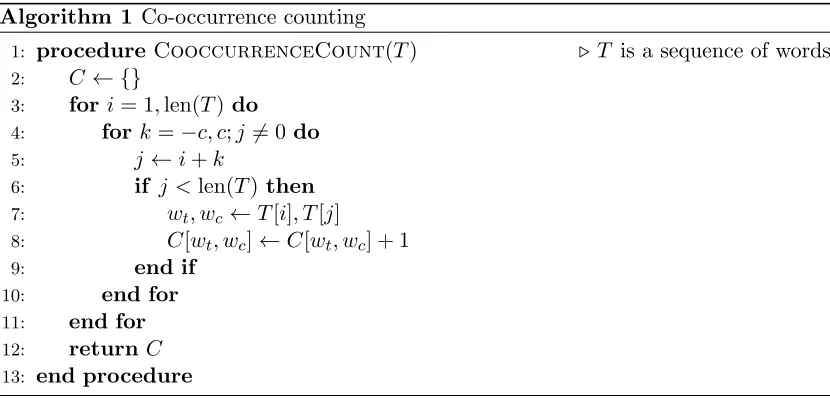
This process produces a matrix of size N×M such as the one in Table 2.1, whereN is the number of targets andM the number of contexts. In this example, the wordplayer

(14)

player field court Athenian king a

baseball 546 350 5 1 35 975

basketball 485 10 410 1 45 1053

democracy 1 5 2 350 10 375

monarchy 2 1 4 7 276 330

Table 2.1: Sample counts of target/context co-occurrences in a text corpus.

In order to highlight infrequent but informative terms, and downplay the role of frequent but uninformative contexts these counts are further transformed with a non-linear

op-eration. By far, the most commonly used transformation is Positive Pointwise Mutual Information or PPMI (Church and Hanks,1990), defined as follows:

PPMI(i, j) = max (PMI(i, j),0) (2.1)

PMI(i, j) = log _P_N ZC[i, j]

k=1C[k, j]

PM

l=1C[i, l]

!

(2.2)

whereZ =PN

k=1

PM

l=1C[k, l] is a normalizing constant.

PMI expresses how much more or less frequent a co-occurrence between two terms is in relation to what you would expect if these where two independent events. PPMI is the truncated version where negative values are discarded. Table 2.2 shows how the counts in the example above look when the PPMI transformation is applied. Notice how random noise is flattened down and non-informative all-present terms like the articlea

gets also discounted.

player field court Athenian king a

baseball 0.38 0.97 0 0 0 0

basketball 0.21 0 0.94 0 0 0.01

democracy 0 0 0 1.93 0 0

monarchy 0 0 0 0 1.86 0.03

Table 2.2: Sample pmi-transformed counts of target/context co-occurrences in a text corpus.

These resulting vectors (taken row-wise) can already be used as the semantic represen-tations of the target words. However, it typically yields some improvement to apply a

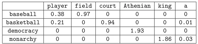
dimensionality reduction technique such as SVD (Landauer and Dumais,1997;Strang,

2003), to obtain compact representations of much smaller dimensionkM.

SVD works by decomposing the original matrix (in this case, the PPMI-weigthed co-occurrence matrix) X ∈ _RN×M _as _X ₌ _{U SV}>_{, where} _U _∈

(15)

matrix; S ∈ _RN×M_{, a diagonal matrix with sorted non-negative values (known as} sin-gular values) in the diagonal and another orthogonal matrix V ∈_RM×M_{. Crucially, by}

computing the outer product between the first column vectors ofU and V, weighted by the first singular value, one can recover as much information from the original matrixX

as it is possible with a rank-1 matrix. Similarly, by adding the second column vectors

weighted by the second singular value one can recover the maximal amount of informa-tion ofX that is possible to express with a rank-2 matrix. In general, one can form the

best rank-k approximation of the original matrix by summing over the firstk principal components, that is, the outer product of the firstkcolumn vectors ofU andV weighted

by their singular values Sii,1≤i≤k. See Figure2.2 for a schematic representation of this

factorization and Figure 2.3, for an example of an image being approximated with the first kprincipal components.

Σ

U S V>

= =

X

=

Figure 2.2: SVD decomposition as a sum of independent components that form the

best rank-kapproximation of a matrix.

When factorizing the semantic vectors matrix, the vectors in U ∈ _RN×N _still

corre-spond to the target words: Multiplied by SV> they would reconstruct the original

M-dimensional vectors. Furthermore, U S is a matrix having the same shape as the original X ∈ _RN×M_{, but expressed in a base where the first columns capture most of}

the original information. Therefore, the typical practice consist in truncatingU S

(16)

(a) Original image (rank 348)

(b)Rank 5 approximation. (c)Rank 30 approximation.

(d) Rank 55 approximation. (e) Rank 80 approximation.

Figure 2.3: Reconstruction of an image using the rank-k approximation given by

SVD.

2.1.2 Predict models

Predict models where first introduced by Bengio et al. (2003), becoming particularly prominent with the word2vec model (Mikolov et al., 2013) thanks to its large-scale efficiency and strong empirical results. Word2vec finds its underlying idea in storing into each word vector the information that allows it to predict its most prototypical

(17)

similar to count models, and indeed, Levy and Goldberg (2014) show that common implementations of the two optimize the same objective function.

The two main models introduced by Mikolov et al. can be construed as shallow neural networks with a single embedding layer and no non-linearity. Under this framework,

words in the target and the context vocabularies get assigned dense vectorsv∈Rdthat

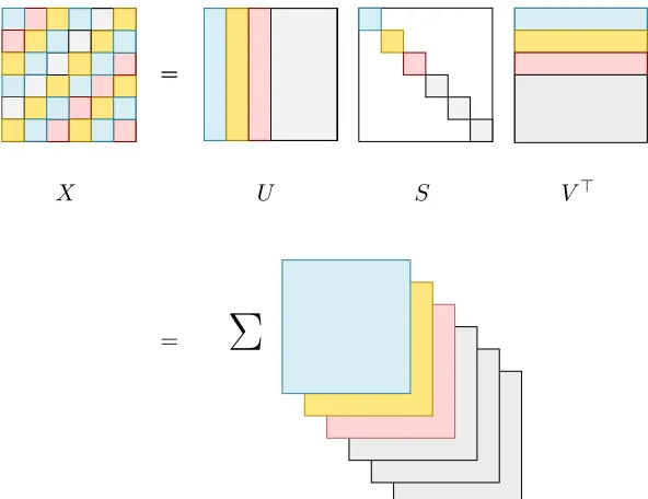
are randomly initialized. Then, the contents of these vectors are adjusted with slightly different prediction objectives depending on the type of model. In the Continuous

Bag-of-Words or CBOW model, the vectors are trained so that the sum of the context vectors best predict the target word (Figure 2.4a) from all the other words in the vocabulary. On the other hand, the Skip-Gram (SG) model, uses the target word as input and tries to predict each of the words in the context.

Question the

of

Ultimate

Life

V ×d d×V

v v0

(a) CBOW model

Question Life of Ultimate the

d×V d×V d×V d×V

V ×d v v0

(b)Skip-Gram model

Figure 2.4: Graphical illustration of the two predict models introduced byMikolov

et al.(2013).

More precisely, the SG objective function is to maximize the log-probability of the context word given the target, for each target-context words pair observed in the corpus:

J(Θ) =

|T|

X

i=1

X

i−c≤j≤i+c,j6=i

logP(wj|wi) (2.3)

where the probability distribution is defined following the Boltzmann distribution1:

P(wj|wi) = exp

v_w0_j ·vwi

PN

w=1exp (vw0 ·vwi)

(2.4)

1

(18)

vwi is the vector corresponding to the given target word wi, while v

0

j is the vector

corresponding to context word wj that must be predicted. The vectors are updated

after observing each word pair in the corpus according to the goal of optimizing the above mentioned objective function, using stochastic gradient descent (SGD).

Observe that what this objective function does is to enforce the dot product between

vectors of co-occurring target-context word pairs to be larger than those of non-co-occurring ones. Also remember that the dot product between two vectors a and b, separated by an angle θ, is defined as:

~a·~b=cos(θ)k~akk~bk (2.5) Therefore, the best way to modify the word vectors such that the dot product between co-occurring pairs (e.g. basketballandplayer) becomes larger, while lower for the others

(e.g. basketballandAthenian) is to push the angle between the vectors corresponding to the first two terms smaller, and larger for the others. This is indeed what SG training

updates achieve, by bringing word vectors’ closer to the ones of their collocates, as illustrated in Figure2.5.

basketball Athenian

player

~vbasketball·~vplayer

~

vbasketball·~vAthenian

Figure 2.5: Sample vector update in a predict-style model when a

basketball/playertarget-context pair is observed. basketballvector is “rotated” in the direction of player’s vector, thus enlarging the dot product between them, while

reducing it with the non-observed contextAthenian.

2.2

Compositional Distributional Semantic Models

In the previous section we have established a mechanism to produce semantic represen-tations to individual words. How can we represent the meaning of larger expressions?

One option would be to proceed exactly in the same way, collecting co-occurrences, this time not for words but for full phrases. However, this approach suffers the problem

of data sparsity: With rare exceptions, such as frequent multi-word expressions in lan-guages like English, the larger the phrase, the less it will be attested in corpora. Even

(19)

Distributional Semantic Models (CDSM), which propose different algebraic operations to compose the meaning of the parts to obtain the meaning of the whole.

Mitchell and Lapata (2010) proposed a set of simple models in which each component of the phrase vector is a function of the corresponding components of the constituent

vectors. Given vectors ~a and ~b, the weighted additive model (wadd) returns their weighted sum: ~p=w1~a+w2~b. In the dilation model (dil), the output vector is obtained

by decomposing one of the input vectors, say ~b, into a vector parallel to ~a and its

orthogonal counterpart, and then dilating only the parallel vector by a factor λbefore re-combining. The corresponding formula is: (~a·~a)~b+ (λ−1)(~a·~b)~a. In our experiments (Chapter3 below), we stretch the head vector in the direction of the modifier (i.e.,~ais the modifier,~b is the head). In the multiplicative model (mult), vectors are combined by component-wise multiplication, such that each phrase component pi is given by:

pi =aibi.

Guevara (2010) and Zanzotto et al. (2010) propose a full form of the additive model (fulladd), where the two constituent vectors are multiplied by weight matrices before being added, so that each phrase component is a weighted sum of all constituent

com-ponents: ~p=W1~a+W2~b.

Finally, the lexical function (lexfunc) model ofBaroni and Zamparelli (2010) and Co-ecke et al. (2010) takes inspiration from formal semantics to characterize composition as function application. In particular, adjective-noun phrases, the adjective is treated as a linear function operating on the noun vector. Given that linear functions can be

expressed by matrices and their application by matrix-by-vector multiplication, the ad-jective is represented by a matrix A to be multiplied with the noun vector~b, so that:

~ p=A~b.

This latter approach is further generalized by Baroni et al. (2014a) to cases in which words must take more than one argument. For example, verbs take the subject and the object as input and return the sentence representation as the output. To account

for these cases, the authors propose to use high-order tensors, which can take as many arguments as allowed by their cardinality. The drawback of this approach is that it involves setting a very high number of parameters. For this reason,Paperno et al.(2014) propose to approximate these tensor operators by a linear combination of matrix-vector multiplication factors, denominated practical lexical function (plf).

(20)

involve the compositional operation that we are trying to estimate. The parameters are then learned through least-squares regression with the objective of approximating the

phrases-observed vectors starting from the representations of their parts. For example, to approximate the lexical function corresponding to the adjectivered, one would compute the corpus-extracted vectors for phrases like red face, red wine, red car, etc., and

then estimate the weights of the mapping, such that, given the vector forface, produces

(21)

Chapter 3

Modification effects in conceptual

hierarchies

“This parrot is no more. It has ceased to be. It’s expired and gone

to meet its maker. This is a late parrot. It’s a stiff. Bereft of life,

it rests in peace. If you hadn’t nailed it to the perch, it would be

pushing up the daisies. It’s rung down the curtain and joined the

choir invisible. This is an ex-parrot!”

— John Cleese, Monty Python’s Flying Circus

3.1

Introduction

Not all modifiers are created equal. Green parrots have all essential qualities of parrots,

but dead parrots don’t. For example, as vocally argued by the disgruntled costumer in Monty Python’s famous Dead Parrot Sketch,1 dead parrots make rather poor pet birds. In modifier-head constructions (that, for the purpose of this chapter, we restrict to right-headed adjective-noun and noun-noun constructions), modifiers are not simply picking a subset of the denotation of the head they modify, but they are oftendistorting

the properties of the head in a radical manner.

These modifier effects on phrase meaning have been studied extensively by theoretical

linguists, who have focused primarily on the extreme case of intensional modifiers such asfake,alleged and toy, where the phrase denotes something that is no longer (or is not

necessarily) a head (a toy gun is not a gun). See McNally (2013) for a recent review of the linguistic literature. Cognitive scientists have looked at modification phenomena

1

http://en.wikipedia.org/wiki/Dead_Parrot_sketch

(22)

Modification effects in conceptual hierarchies 14

within the general study of conceptual combination (see Chapter 12 of Murphy(2002) for an extensive review). The cognitive tradition has focused on how modification affects

prototypicality: a guppy is the prototypical pet fish, but it is neither a typical pet nor a typical fish (Smith and Osherson, 1984). This line of research has highlighted how strong modification effects might be the rule, rather than the exception: Wisniewski

(1997) reports that, when subjects were asked to provide the meaning for more than 200 novel modifier-head constructions, “70% [of the answers] involved the construal of

a noun’s referent as something other than the typical category named by the noun [head].” Indeed, recent research suggests that even the most stereotypical modifiers

affect prototypicality, so that subjects are less willing to attribute to quacking ducks

such obvious duck properties ashaving webbed feet (Connolly et al.,2007).

The impact of modification on phrase meaning is not only very interesting from a

lin-guistic and cognitive perspective, but also important from a practical point of view, as it might affect expected entailment patterns: If parrot entails pet, then lively parrot

also entails pet. However, as we saw above, dead parrot doesn’t necessarily entail pet

(at least not from the point of view of a disgruntled costumer who was just sold the

corpse). Being able to track the impact that modifiers have on heads should thus have a positive effect on important tasks such as recognizing textual entailment, paraphrasing and anaphora resolution (Androutsopoulos and Malakasiotis, 2010; Dagan et al., 2009;

Poesio et al.,2010).

Despite their theoretical and practical import, modification effects have been largely

overlooked in computational linguistics, with the notable exception of Boleda et al. (Boleda et al.,2012,2013), who only focused on the extreme case of intensional adjectives, stud-ied a limited number of modifiers, and did not attempt to capture the graded nature

of modification (a dead parrot is not a prototypical animal, but a toy parrot is not an

animal at all).

In this Chapter, I will describe how we have built a large, publicly available data set of modifier-head phrases annotated with four kinds of modification-related subject ratings:

whether the concept denoted by the phrase is an instance of the concept denoted by its head (is a dead parrot still a parrot?), to what extent it is a member of one of the larger categories the head belongs to (is it still a pet?), and typicality ratings for the

same questions (how typical is a dead parrot as a parrot? and as a pet?).

Second, I will present our efforts to model the collected judgments computationally

using DSM. In particular, we look at the compositional extension of distributional se-mantics, because we need representations not only for words, but also phrases, and we

(23)

an asymmetric relation (to what extent the concept denoted by the phrase is a good instance of the target class, and not vice versa). As far as we know, this is the first

time these asymmetric measures are applied to composed representations (Baroni et al.

(2012) experimented with entailment measures applied to phrase representations directly harvested from corpora, and not derived compositionally).

The setup of the task involves producing fine-grained inferences that make intensive use of human conceptual knowledge, both from the compositional side and the hierarchical

organization side. We are thus evaluating distributional representations on a challenging setting where they could also potentially be very useful.

3.2

The Norwegian Blue Parrot data set

We introduce Norwegian Blue Parrot (NBP),2 a new, large data set to explore modifi-cation effects. Given ahead nounh and amodifier adjective or nounm, NBP contains average membership and typicality ratings for the phrase mhboth as an instance of h

and as an instance ofc (a broadercategoryhbelongs to). As a control, we also present ratings for unmodified h as an instance of c (we will use them below to test similarity

measures on their ability to capture the direction of the membership relation, and to zero in on the effect of modification vs. more general membership/typicality effects). We

include, and indeed focus on, relations with broader categories because they are more prone to modification effects: Intuitively, a dead parrot is still a parrot, but it is, at the very least, an atypical pet. The statistics in Table 3.1, discussed below, confirm our intuition that subjects are more likely to assign lower scores with respect to a broader category than to the head category itself (although this is, no doubt, in part by

con-struction, since we started constructing the dataset by mining examples where mh is atypical of c, not h). We collect both membership and typicality ratings because we expect them to have different implications for sound entailment. If x is not a member

of class y, thenx obviously does not entaily. However, ifx is an atypicaly, entailment still holds, but some typical properties of y might not carry over (e.g., in an anaphora

resolution setting, we might still consider co-indexingdead parrot with animal, but not withbreathing creature, despite the fact thatbreathing is a highly characteristic property

of animals).

In order to make sure that NBP would contain a fair number of examples affected

by strong modification effects, we first came up with a set of hm, h, ci tuples where, according to our own intuition, m makes h fairly atypical as an instance of c. For example, abottleis a piece ofdrinkware. If we add the modifierperfume, we expect that,

2

(24)

while subjects might still agree that a perfume bottle is a bottle, they should generally disagree on the statement that a perfume bottle belongs to thedrinkware category. We

refer to tuples of this sort (e.g., hperf ume, bottle, drinkwarei) as distorted tuples in what follows.3

We then constructed a number of tuples that should not display a strong modification effect. In particular, in order to insure that any atypical rating we obtained on the distorted tuples could not be explained away by characteristics of m orh alone (rather

than by their combination), for each distorted tuple we constructed a few more tuples with the samehandcbut a differentm, that we did not expect to be strongly distorting

(e.g.,hplastic, bottle, drinkwarei). Similarly, for each distorted tuple we generated a few more with the same m, but combined with (the same or different) h and c on which them should not exert a strong effect (hperf ume, bottle, containeri). In total, NBP is based on 489 distorted tuples and 1938 more matching tuples.

We constructed NBP to insure that it would contain many tuples displaying strong

modification effects, and highly comparable tuples that do not feature such effects. An alternative approach would have been to rate phrases that were randomly selected from

a corpus. This would have led to a dataset reflecting a more realistic distribution of modification effects, but it would not have guaranteed, for the same number of pairs,

a fair amount of distorted tuples and comparable controls. We leave the study of the natural distribution of modification strength in text to further work.

To find inspiration for the tuples, we looked into various databases containing concepts

organized by category, namely BLESS (Baroni and Lenci,2011), ConceptNet (Speer and Havasi,2013) and WordNet (Fellbaum, 1998). We insured that all words in our tuples occurred at least 200 times in the large corpus we describe below (phrases were not filtered by frequency, due to data sparseness). Finally, when looking for tuples matching

the distorted ones, we made sure that the mh phrases in the new tuples have similar Pointwise Mutual Information to the corresponding phrases in the distorted tuple (or, where the latter were not attested in the corpus, similarm andh frequencies). Finding

meaningful combinations among unattested or infrequent phrases was not an easy task and there was not always a perfect candidate. However, the phrases selected in this way

yielded challenging items for which there is little or no direct corpus evidence, so that compositional models are required to account for them.

From each source tuple (e.g.,hplastic, bottle, drinkwarei), we generated 3 instance-class combinations to be rated: mh→c(plastic bottle →drinkware),mh→h (plastic bottle

3

(25)

→ bottle), h → c (bottle → drinkware), for a total of 5,849 pairs, that constitute the final NBP data set (2,417 mh→c pairs, 2,115mh→h pairs and 1,317 h→cpairs).4 For each of these pairs, we collected both membership and typicality ratings through two surveys on the CrowdFlower platform.5 Subjects came exclusively from English speaking countries and no special qualifications were required from them. Membership ratings were collected by asking subjects whether the instance is a member of the class (formulated as a yes/no question). In a separate study, we asked subjects to rate how

typical the instance is as member of the class on a 7-point scale. For both questions, we collected 10 judgments per pair and report their averages in NBP. For both surveys,

we added 48 control pairs with an expected answer (yes/no for membership, high/low range for typicality), that the subjects had to provide in order for their ratings to be included in the final set (“gold standard” items in crowd-sourcing parlance). These

controls included highly prototypical pairs (dog →animal), possibly with stereotypical modifiers (beautiful rose →flower), and unrelated pairs (biology →dance), also possibly under modification (popular magazine → animal).

We asked for binary rather than graded membership judgments because these are more

in line with commonsense intuitions about category membership (we might naturally speak of sparrows being more typical birds than penguins, but it is strange to say that

they are “more birds”). The standard view in the psychology of concepts (Hampton,

1991) is that membership judgments are the product of a hard threshold we impose on the typicality scale (x is not y if the typicality of x as y is below a certain,

subject-dependent threshold), although under certain experimental conditions subjects can also conceptualize membership as a graded property (Kalish,1995).

Membership and typicality ratings, especially in borderline cases such as those we con-structed, are the output of complex cognitive processes where large inter-subject

differ-ences are expected, so it doesn’t make sense to worry about “inter-annotator agreement” in this context. Still, several sanity checks indicate that, overall, our subjects understood our questions as we meant them, and behaved in a reasonably coherent manner. First,

both average membership and typicality, ratings are significantly lower (p < 0.001) for themh→cpairs deriving from those tuples that we manually labeled as distorted than for the non-distorted ones. Moreover, for membership, in 86% of the cases at least 8 over 10 subjects gave the same response. For typicality, the observed average rating standard

deviation across pairs (1.2) is significantly below what expected by chance (p <0.05), based on a simulated random rating distribution. Membership and typicality ratings are highly correlated, but not identical (r = 0.76)

4

There is a larger number ofmh→cpairs because different tuples can lead to the samemh→hor

h→ccombinations. 5

(26)

Table 3.1 reports mean membership and typicality scores in NBP. Both ratings are negatively skewed, that is, subjects had the tendency to respond assertively to the

membership question and to give high typicality scores. This is not surprising: Because of the way NBP was constructed, there are about 4 tuples with no expected strong modification effect for each distorted tuple. Furthermore, except for the negative control

items (not entered in NBP), our questions did not feature cases where a negative/low response would be entirely straightforward (of the “is a cat a building?” kind). We

observe moreover that, in accordance with the intuition we discussed at the beginning of this section, the ratings are extremely high when the class is identical to the phrase

head. On the other hand, the mh → c condition displays, as expected, the lowest averages, suggesting that this will be the most interesting type to model experimentally.

measure mh→c mh→h h→c tot.

memb. 0.84 (0.2) 0.97 (0.1) 0.88 (0.2) 0.89 (0.2)

typ. 5.45 (1.1) 6.29 (0.6) 5.81 (1.0) 5.84 (1.0)

Table 3.1: NBP summary statistics: Mean average ratings and their standard devi-ations across pairs, itemized by instance-class type and in total. Membership values

range from 0 to 1, typicality values from 1 to 7.

Table 3.2 presents a few example entries from NBP. The first block of the table illus-trates cases with the highest possible membership and typicality scores. At the other

extreme, the second block contains examples with very low membership and typicality. Interestingly, there are also cases, such as the ones in the third block of the table, where all subjects agreed on class membership, but the typicality scores are relatively low (we

did not find clear cases of the opposite pattern, and indeed we would have been surprised to find highly typical instances of a class not being treated as members of the class).

Some examples in Table 3.2 illustrate an important design choice we made in con-structing NBP, namely, to ignore the issue of whether potential modification effects are actually due to the modifier and the category pertaining to differentword senses of the

head term. One might argue, for example, thategg has afood sense and areproductive vessel sense. Thehuman modifier picks the second sense, and so, obviously,human eggs

are judged as bad instances of food. While we see the point of this objection, we think

it’s impossible to draw a clear-cut distinction between discrete word senses (even in the rather extreme egg case, the eggs we eat are reproductive vessels from a chicken point

(27)

instance class memb. typ.

top membership, top typicality gourmet soup food 1.00 7.00

huge tiger predator 1.00 7.00 sugared soda drink 1.00 7.00 live fish animal 1.00 7.00 Thai rice rice 1.00 7.00 silver spoon spoon 1.00 7.00

low membership, low typicality fatal shooting sport 0.20 1.40

human egg food 0.40 1.50 perfume bottle drinkware 0.10 1.30 explosive vest commodity 0.30 1.90 lemon water chemical 0.20 1.60 creamy rice bean 0.20 1.30 top membership, (relatively) low typicality

sick tuna tuna 1.00 3.20 explosive vest vest 1.00 3.50 perforated sieve tool 1.00 4.20 bottled oxygen substance 1.00 4.30 grilled trout creature 1.00 4.40 educational toy amusement 1.00 4.50

Table 3.2: Instance-class pairs illustrating various combinations of membership and typicality ratings in NBP.

provides fundamental cues to disambiguating polysemous words, and noun modifiers

typically act as important disambiguating contexts for the nouns. Thus, we think that it is more productive for computational systems to handle modifier-triggered

disam-biguation as a special case of the more general class of modification effects, than to engage in the quixotic pursuit to determine, a priori, what’s the boundary between a word-sense and a “pure” modification effect. Note in Table 3.2 that grilled trout was unanimously rated by subjects as an instance of the creature category, despite the fact that the cooking-related grilled modifier cues a classic shift from an animal (and thus

creature) sense tofood (Copestake and Briscoe, 1995). Examples like this suggest that our agnosticism is warranted.

3.3

Methods

3.3.1 Composition models

We experiment with many ways to derive a phrase vector by combining the vectors of

its constituents. In particular, we explore the wadd,dil, mult, fulladd and lexfunc

(28)

We use the DISSECT toolkit6 to estimate the parameters of the composition methods and derive phrase vectors. In particular, DISSECT finds optimal parameter settings

by learning to approximate corpus-extracted phrase vector examples with least-squares methods (Dinu et al.,2013). We use as training examples all the modifier-head phrases that contain a modifier of interest and occur at least 50 times in our source corpus (see

Section3.3.3below).

3.3.2 Asymmetric similarity measures

Several measures to identify word pairs that stand in an instance-class relationship by

comparing their vectors have been proposed in the recent distributional semantics lit-erature (Kotlerman et al., 2010;Lenci and Benotto,2012;Weeds et al.,2004).7 While the task of deciding if u is in class v is typically framed (also by distributional

seman-ticists) in binary, yes-or-no terms, all proposed measures return a continuous numerical score.8 Consequently, we conjecture that they might be well-suited to capture the graded notions of class membership and typicality we recorded in NBP.9

In what follows, we usewx(f) to denote the weight (value) of feature (dimension) f in

the distributional vector of term x. Fx denotes the set of features (dimensions) in the vector of x such that wx(f) > t, where t is a predefined threshold to decide whether a

feature is active.10 _{Importantly, all measures assume non-negative values.}

Most asymmetric measures proposed in the literature build upon thedistributional in-clusion hypothesis, stating that “if u is a semantically narrower term than v, then a

significant number of salient distributional features ofuis included in the feature vector ofv as well” (Lenci and Benotto,2012). In our terminology, uis the potential instance, and v is the class. We re-implement all the measures adopted by Lenci and Benotto, namely weedsprec, cosweeds, clarkede and invcl (see their paper for the original references):

6

http://clic.cimec.unitn.it/composes/toolkit/

7_{We speak of “instance-class relations” in a very broad and loose sense, to encompass classic relations} such as hyponymy but also the fuzzier notion of lexical entailment.

8_{SVM classifiers have also been shown by}_{Baroni et al.}₍₂₀₁₂_{) to be well-suited for entailment} detec-tion, but they do not naturally return continuous scores.

9_{Subjects had to answer a yes/no question concerning class membership, but by averaging their} response we derive continuous membership scores.

10_{The obvious choice for}_t_{is 0. However, when working with the low-rank spaces described in Section}

(29)

weedsprec(u, v) =

P

f∈Fu∩Fvwu(f) P

f∈Fuwu(f)

(3.1)

cosweeds(u, v) =pweedsprec(u, v)×cosine(u, v) (3.2)

clarkede(u, v) =

P

f∈Fu∩Fvmin(wu(f), wv(f)) P

f∈Fuwu(f)

(3.3)

invcl(u, v) =pclarkede(u, v)×(1−clarkede(u, v)) (3.4)

The cosweeds formula combines weedsprec with the widely used symmetriccosine mea-sure:

cosine(u, v) =

P

f∈Fu∩Fvwu(f)×wv(f) q

P

f∈Fuwu(f)

2_×qP

f∈Fvwv(f)

2

(3.5)

Finally, we experiment with the carefully craftedbalapincmeasure of Kotlerman et al.

(2010):

balapinc(u, v) =plin(u, v)·apinc(u, v) (3.6)

where thelin term is computed as follows:

lin(u, v) =

P

f∈Fu∩Fvwu(f) +wv(f) P

f∈Fuwu(f) + P

f∈Fvwv(f)

(3.7)

The balapinc score is the geometric average of a symmetric similarity measure (lin) and

(30)

3.3.3 Distributional semantic spaces

We use count models to produce our distributional vectors because their determinis-tic training procedure makes it easier to train compositional models. We extract

co-occurrence information from a corpus of about 2.8 billion words obtained by concate-nating ukWaC,11 Wikipedia12 and the British National Corpus.13 With DISSECT, we build co-occurrence vectors for the top 20K most frequent lemmas in the source corpus (plus any NBP term missing from this list). We treat the top 10K most frequent lemmas as context elements. We consider context windows of 2 and 20 words on the two sides of

the targets. We weight the vectors by non-negative Pointwise Mutual Information and Local Mutual Information (Evert, 2005). We experiment with vectors in the resulting full-rank (10K-dimensional) semantic spaces as well as with vectors in spaces of ranks 100 and 300. Rank reduction is performed by applying the Singular Value Decomposi-tion (Golub and Van Loan,1996) or Non-negative Matrix Factorization (Lee and Seung,

2000). It is customary to represent the output of these operations directly in a dense low-dimensional space. However, the asymmetric similarity measures we use assume

sparse vectors (or the “inclusion” criterion would be meaningless), so we project back the outcome of SVD and NMF to sparse 10K-dimensional but low-rank spaces. In total,

we explore 20 distinct semantic spaces.

We also collect co-occurrence vectors for the phrases needed to estimate the composition

method parameters (see Section 3.3.1 above). We use DISSECT’s “peripheral space” option to project the phrase raw count vectors into the various spaces without affecting their structure.

Due to memory constraints, we restrict evaluation in the full-rank spaces to the wadd

and mult models.

3.4

Experiments

Given the methods described above, the main question we want to answer is: Which combination of compositional model and asymmetric similarity measure yields a better

fit for the data in the NBP dataset?

We start however with a sanity check on the ability of the measures to capture the

direction of the instance-class membership relation. Even a measure that is good at

11_{http://wacky.sslmit.unibo.it} 12

http://en.wikipedia.org 13

(31)

capturing degrees of membership/typicality won’t be of much practical use if it is not able to tell us which item in a pair is the instance and which is the class.

Detecting membership direction As described in Section 3.2 above, NBP also contains single-word h→c pairs (parrot→pet). We extracted the subset of those that all judges considered to be in the category membership relation, and we checked them

manually to make sure that the direction was one-way only. This resulted in a set of 639 pairs where the membership relation holds unidirectionally. We tested all combination

of semantic spaces (Section 3.3.3) and asymmetric similarity measures (Section 3.3.2) on the task of assigning a higher score to the pairs in the h → c (vs. c→ h) direction (e.g., (score(parrot→pet)> score(pet →parrot)). Table 3.3reports, for each measure, the number of spaces in which the measure was able to predict membership direction significantly better than chance (binomial test,p <0.05). We report results on full- and

low-rank (SVD, NMF) spaces separately since, as discussed above, for most composition models we can only use the latter. We observe that all measures are able to significantly

detect directionality in at least some spaces. For all the analyses below, we exclude from further testing the space-measure combinations that failed to pass this sanity check, since they are clearly failing to capture properties pertaining to the instance-class relation (if

a combination is not able to tell that it is aparrot that is apet, and notvice versa, there is no point in asking if the same combination is able to model how typical adead parrot

is as apet).

clarkede weedsprec balapinc cosweeds invcl

Low-rank spaces

10 8 11 8 7

Full-rank spaces

2 4 4 4 2

Table 3.3: Number of spaces (over totals of 16 low-rank and 4 full-rank spaces) in

which each measure was able to predict class membership direction significantly above chance.

Modeling typicality ratings of mh→ c pairs Next, for each of the remaining spaces, we first performed composition as described in Section 3.3.1 above to build the representations for the nominal phrases in the NBP dataset, and then computed asymmetric similarity scores for pairs made of a phrase and the corresponding potential class.

We computed the correlations between mean human membership or typicality ratings and the scores produced with each combination of composition model, similarity measure

(32)

highly correlated (r = .99), and we thus report only the latter. We leave it to further work to devise measures that are more specifically tuned to capture membership or

typicality.

Table3.4reports the top correlation coefficients between typicality judgments and scores of eachmh→cpair (dead parrot→pet) across spaces, organized by measures and compo-sition methods. The best correlation is achieved with the weedsprec measure using the mult composition model in a full-rank space (precisely that of context window size 2 and

ppmi weighting). Recall that mult returns the component-wise product of the vectors it combines. Thus, modification under mult is carried out by picking only those features

of the head that are also present in the modifier, and enhancing them by a factor given by the modifier’s feature value. The weedsprec measure is then given by the weighted proportion of active features in mh that are also active in c. Therefore, the more the

modifier shares features with the parent category, the higher weedsprec will be. This might explain why weedsprec is a good fit for the mult model in measuring degrees of

category typicality.

Looking at composition methods, there is no evidence that the more complex,

matrix-based fulladd and lexfunc approaches are performing any better than the simple mul-tiplicative and additive methods. Indeed, mult shows the most consistent overall

per-formance, confirming the conclusion of Blacoe and Lapata (2012) that, at the present time, when it comes to composition, “simpler is better”. A related point emerges from the comparison of the low- and full-rank results for mult and wadd. The smoothing

process due to dimensionality reduction is quite disruptive for the current asymmetric measures, that are based on feature inclusion. This is a further reason to stick to simpler

composition methods, that can be applied directly in the full-rank spaces.

Regarding the measures themselves, we see that cosweeds, that balances weedsprec with

the classic cosine score, is the most robust, returning good results across all composition methods. On the other hand, the related clarkede and invcl measures turn out to be quite brittle.

The highly significant correlations show that the measures do capture to some extent the patterns of variance in the data. However, when considering potential practical

applica-tions, even the highest reported correlation (.39) is certainly not impressive, indicating that there is plenty of room for further research into developing better composition

methods and/or membership/typicality measures.

Focusing on the modifier effect for mh→c pairs The typicality judgment for

(33)

Low-rank spaces

dil 9* 15* 16* 19* 8*

fulladd 17* 16* 12* 24* −3

lexfunc 17* 12* 12* 27* −2

mult 13* 19* 19* 29* 12*

wadd 14* 14* 16* 27* −2

Full-rank spaces

mult 9* 39* 33* 36* 15*

wadd 30* 34* 31* 35* 14*

Table 3.4: Percentage Pearsonrbetween asymmetric similarity measures andmh→c typicality ratings. *p <0.001

Low-rank spaces

dil 5 −1 −1 −2 7*

fulladd 10* 7* 5+ 7+ −2

lexfunc 15* 9* 10* 18* −2

mult 4+ 14* 13* 15* 9*

wadd 7+ 7* 9* 12+ −2

Full-rank spaces

mult 1 25* 21* 24* 5+

wadd 11* 18* 13* 20* 2

Table 3.5: Percentage Pearsonrbetween asymmetric similarity measures andmh→c

typicality ratings whereh→cscores have been partialed out. *p <0.001, +p <0.05

how much more or less typicaldead parrots are aspets, as opposed toparrots in general. A good model must be able to capture both factors (and this is what we tested above).

However, we are also interested in assessing to what extent the models are capturing the modification effectproper, as opposed to the overall degree of typicality of the h

concept as member of the ccategory. To focus on the modification factor, we partialed out theh→c (parrot→pet) ratings from the mh→c(dead parrot→pet) ratings and from the corresponding model scores (that is, we correlated the residuals of mh→c ratings and model-produced scores after regressing the h→c ratings on both). The results are shown in Table 3.5. Correlations are lower overall, but the general picture from the previous analysis still holds, confirming that the computational models are (also) capturing modifier effects. Interestingly, wadd, dil and fulladd generally undergo larger

performance drops than mult and lexfunc. Evidently, models like the latter, in which the modifier selects the relevant features from the head, are better suited to explain

modification than the former, in which the modifier features are just added to those of the head by means of a linear combination.

(34)

Low-rank spaces

dil 2 −1 −2 −3 4

fulladd 5+ 5+ 2 1 −1

lexfunc 14* 8* 14* 17* −1

mult 3 - 13* 15* 5+

wadd 6+ 8* 7+ 6 −3

Full-rank spaces

mult −2 - 18* 19* −2

wadd 7* 13* 7* 12* −2

Table 3.6: Percentage Pearsonrbetween asymmetric similarity measures andmh→h typicality ratings. *p <0.001, +p <0.05

Section3.2, when the very same concept is used as phrase head and category, judgments are subject to a strong ceiling effect, and none of our measures is designed to flatten out above a certain threshold. Indeed, if we measure the skewness of the typicality

ratings,14 we obtain that, while forh→cand mh→cthe skewness is of−1.9 and−1.5, respectively, formh→h it gets to−3.9.

In any case, the results confirm the brittleness of the clarkede and invcl measures. The linguistically motivated lexfunc model emerges here as a competitive alternative to the simpler models. Still, the best results are obtained with mult and cosweeds (on the

full-rank, context window size 20, ppmi weighted space). Notably, weedsprec applied to a pair of the type mh→ h, where the phrase is constructed using the mult model, results in a constant value of 1, whatever the modifier and the head noun is. This is due to the fact that the features of a phrase composed using mult are a subset of the

features of the head,15and in this case the head is the same as the category. Therefore, by definition, weedsprec yields a score of 1 for every pair, the variance is null and hence the correlation is undefined. As a consequence, in this case cosweeds, which is

the geometric mean between weedsprec and cosine, reduces to cosine similarity! The latter might be effective in capturing the degree of similarity between the phrase and its

potential category but, as a symmetric measure, it cannot, alone, provide a full account of category typicality effects.

14

A skewness factor of 0 means that the distribution is balanced around the mean, while the more negative the coefficient is, the more the left tail is longer and the distribution is concentrated to the right (toward high typicality values in our case).

15

(35)

3.5

Conclusion

We introduced the challenge of quantifying the impact of modification on the meaning

of noun phrases, presenting a new dataset that collects membership and typicality rat-ings for modifier-head phrases with respect to the category represented by the head as

well as a broader category. Since accounting for modifier distortion requires semantic representations of phrases and modeling graded judgments, we consider this an ideal

testbed for compositional distributional semantics.

In the interaction between compositional models and directional similarity measures, we

have observed that simpler models yield better results. Specifically, mult and wadd are economical composition models than can be applied on full-rank spaces, which in turn work best with our similarity measures.

Psychologists studying modification effects in concept combination have proposed mod-els that are usually quite complex, relying on hand-crafted feature definitions and making

very strong assumptions about the combination process (see for exampleCohen and Mur-phy (1984),Smith et al. (1988)). Some of these assumptions have led other researchers to argue that prototypes do not compose at all (Connolly et al.,2007). In contrast, the approach we borrow from distributional semantics, while only mildly successful for now, has the advantage of being very simple both in its construction and application, and in

the assumptions that it makes.

Also notable is that we are putting under the same umbrella tasks that have been

traditionally tackled separately. For example, among the effects present in the dataset, we can find both word sense disambiguation (see discussion at the end of Section3.2) and whatMurphy(2002) calls “knowledge effects” (e.g., aplanemakes a very goodmachine, but a paper plane doesn’t). Moreover, these effects can also interact (people know that ahuman egg is actually a single, small cell, and hence not even cannibals would consider

it satisfactory food). We can thus explore the empirical question of whether all these related phenomena can be tackled together, with a single model accounting for all of

them.

In conclusion, the challenge that we introduced brings together concept combination and

non-subsective modification phenomena studied in psychology and theoretical linguistics, and tries to handle them with the standard machinery of computational linguistics. This challenge has proved quite difficult for current tools, but this is exactly what we expected

in the first place. Our goal, from the outset, was to create a task that could help us delimiting the boundaries of computational methods for characterizing human concepts,

(36)

Chapter 4

Boolean Distributional Semantic

Models

“You need Boolean structure.”

— Denis Paperno

4.1

Introduction

You might have never heard of a jabuticaba before. Nevertheless, if I tell you that it is a type of fruit, then you will probably be able to infer many of its properties. This simple example demonstrates the value of a hierarchical organization of concepts. Yet,

regardless of some proposals such as the asymmetric measures we have relied upon in the last chapter, it is still unclear how can we account for such organization in DSMs.

More generally, we would like to be able to detect an entailment relation between two distributed representations of arbitrary linguistic expressions.

In formal semantics, entailment is well-characterized as an inclusion relation between

the sets (of the relevant type) denoted by words or other linguistic expressions, e.g., sets of possible worlds that two propositions hold of (Chierchia and McConnell-Ginet,2000, 299). In finite models, a mathematically convenient way to represent these denotations

is to encode them inBoolean vectors, i.e., vectors of 0s and 1s (Sasao,1999, 21). Given all elements ei in the domain in which linguistic expressions of a certain type denote,

the Boolean vector associated to a linguistic expression of that type has 1 in positioniif

ei∈S forS the set denoted by the expression, 0 otherwise. An expressionaentailing b

will have a Boolean vector including the one ofb, in the sense that all positions occupied by 1s in thebvector are also set to 1 in theavector. Very general expressions (entailing

(37)

Boolean Distributional Semantic Models 29

nearly everything else) will have very dense vectors, whereas very specific expressions will have very sparse vectors. The negation of an expression awill denote a “flipped”

version of the a Boolean vector. Vice versa, two expressions with at least partially compatible meanings will have some overlap of the 1s in their vectors; conjunction and disjunction are carried through with the obvious bit-wise operations, etc.

Despite all these theoretical advantages, formal models lack the large-scale inductive power of distributional semantic models. To narrow the gap between the two, we create

Boolean meaning representations that build on the wealth of information inherent in dis-tributional vectors of words (and sentences). More precisely, we use word (or sentence)

pairs labeled as entailing or not entailing to train a mapping from their distributional representations to Boolean vectors, enforcing feature inclusion in Boolean space for the entailing pairs. By focusing on inducing Boolean representations that respect the

inclu-sion relation, our method is radically different from recent supervised approaches that learn an entailment classifier directly on distributional vectors, without enforcing

inclu-sion or other representational constraints. We show, experimentally, that the method is competitive against state-of-the-art techniques in lexical entailment, improving on them

in sentential entailment, while learning more effectively from less training data. This is crucial for practical applications that involve bigger and more diverse data than the focused test sets we used for testing. Moreover, extensive qualitative analysis reveals

several interesting properties of the Boolean vectors we induce, suggesting that they are representations of greater generality beyond entailment, that might be exploited in

further work for other logic-related semantic tasks.

4.2

Related work

Entailment in distributional semantics Due to the lack of methods to induce

the relevant representations on the large scale needed for practical tasks, the Boolean structure defined by the entailment relation is typically not considered in efforts to au-tomatically recognize entailment between words or sentences (Dagan et al.,2009). On the other hand, some researchers relying on distributional representations of meaning have attempted to apply various versions of the notion of feature inclusion to entailment

detection. This is based on the intuitive idea – the so-called distributional inclusion hypothesis – that the features (vector dimensions) of a hypernym and a