The implementation of the mortar spectral element discretization of the heat equation with discontinuous diffusion coefficient

R E S E A R C H

Open Access

The implementation of the mortar spectral

element discretization of the heat equation

with discontinuous diffusion coefficient

Mohamed Abdelwahed

_{and Nejmeddine Chorfi}

*_{Correspondence:} nchorfi@ksu.edu.sa 1_{Department of Mathematics,}

College of Sciences, King Saud University, Riyadh, Saudi Arabia

Abstract

We propose to implement the mortar spectral elements discretization of the heat equation in a bounded two-dimensional domain with a piecewise continuous diffusion coefficient. The discretization on time is based on the Euler implicit method. Some numerical experiments and comparisons are performed on whether a

conforming or a not conforming domain decomposition.

Keywords: Heat equation; Euler method; Mortar spectral element method; Implementation

1 Introduction

This paper is devoted to the implementation of the discretization by the mortar spectral elements method of the heat equation. We will consider the diffusion coefficient to be piecewise constant and the quotient of its maximal and minimal value to be sufficiently large. The a priori and a posteriori analysis of the heat equations was addressed in a va-riety of work [1–4]. The discretization by the conforming finite element method of the stationary case of the aforementioned heat equation problem was considered in [5]. The same problem was handled by the mortar method for the spectral elements discretization in [6].

In this work, we consider the nonstationary problem. The Euler implicit method is used for the time discretization then a first decomposition of the domain is proposed such that on each sub-domain the diffusion coefficient is constant. A second decomposition is also used based on the mortar method [7], which is the most suitable one for this type of problem, since it is about nonconforming geometries (i.e. it is not necessarily that the intersection of two sub-domains is a corner or a whole edge of both of them) [8]. The non-conforming property permits to reduce the number of sub-domains enormously. Spectral discretization is performed in each sub-domain where the solution is approached by a high degree polynomial. The sub-domains are chosen as rectangles to benefit from the tensorization property of the polynomial basis. The mortar spectral elements method has two advantages. The first one is the possibility to choose polynomial degrees in each sub-domain different from each others. This allows us to take a high degree polynomial in the sub-domains where the value of the diffusion coefficient is large. The second advantage is

that the error estimation depends on the local regularity of the solution rather than on the global regularity. The global regularity of the solution is poor due to the discontinuity of the diffusion coefficient [5,9,10]. This justifies the choice of the domain decomposition method to solve our problem [11]. Some numerical experiments are described. They are fairly coherent with the analysis and support the choice of the mortar method. We refer to [12] for similar numerical results in the mortar h-p version of the finite element method. The outline of this paper is as follows: Sect.2 is devoted to the continuous problem and some regularity results. Section3describes the semidiscrete time problem and the full discrete problem. The error estimation is presented in Sect.4. Finally, Sect.5is ded-icated to the discrete problem implementation. We perform and discuss some numerical experiments.

2 The continuous problem and regularity results

LetΩan open and bounded connected two-dimensional domain with a Lipschtiz contin-uous boundary∂Ω. We consider the following problem, which models the heat equation with a diffusion coefficientλ, depending on the heterogeneity of the domain and not de-pending on time:

⎧ ⎪ ⎪ ⎨ ⎪ ⎪ ⎩

∂ϕ

∂t –div(λgradϕ) =f inΩ×]0,T[, ϕ= 0 in∂Ω×]0,T[,

ϕ(·, 0) =ϕ0 onΩ,

(1)

whereTis a fixed positive real.

We denote in the following by x = (x,y) the elements ofR2_{. We assume that there exist} a finite number of sub-domainsΩ_i, 1≤i≤I, such that:

(1)

Ω= I

i=1

Ω_i, Ω_i∩Ω_j=∅, 1≤i<j≤I;

(2) the restriction ofλto eachΩ_i is continuous onΩ_i,1≤i≤I; (3) λis bounded on eachΩ_i, and we define

λmax= max

1≤i≤Iλ max

i , and λ

min = max

1≤i≤Iλ min

i , (2)

where

λmax_i = sup

x∈Ω_i

λ(x), and λmin_i =min

x∈Ω_i λ(x).

LetHs_{(Ω),s> 0, the Sobolev spaces with the associated norm·}

s,Ωand seminorm|·|s,Ω. The spaceH01(Ω) denotes the closure inH1(Ω) of the space of infinitely differentiable functions with compact support inΩ andH–1_{(Ω) is its dual space. We designate by (·,·)} and · 0,Ω, respectively, the scalar product ofL2(Ω) and its associated norm.

• Cj_{(0,T;X)is a Banach space for the norm}

u_Cj_(0,T;X)= sup

0≤t≤T j

l=0 ∂_tlu_X,

where∂_tluis the derivative of orderlin time of the functionu. It represents the set of classCj_{time-dependent function with a value on a separable Banach spaceX.}

• Lp_{(0,T;X) ={vmesurable on]0,T[such that} T

0 v(t)

p

Xdt<∞}is a Banach space

for the norm

vLp_(0,T;X)=

⎧ ⎨ ⎩

( ₀Tv(t)p_Xdt)1p_{, for1}≤_{p< +}∞_,

sup_0≤t≤Tv(t)X, forp= +∞,

• Hs_{(0,T;X) ={v∈L}2_(0,T;X);∂k_v∈L2_{(0,T;X);k≤s}is an Hilbert space for the scalar}

product:

(u,v) =

(u,v)L2_(0,T;X)+ s

k=0

∂ku,∂kv_L2_(0,T;X) 1

2 .

Problem (1) has the following equivalent formulation:

Fort∈]0,T[ andf ∈L2_(0,T;H–1_{(Ω)), findϕ∈C}0_(0,T;L2_(Ω))∩L2_(0,T;H1

0(Ω)) such that: for allψ∈H1

0(Ω)

Ω ∂ϕ

∂t(x,t)ψ(x)dx+

I

i=1

Ω_i

λ(x)∇ϕ(x,t)∇ψ(x)dx=f(·,t),ψ (3)

where·,·denotes the duality product ofH₀1(Ω) andH–1(Ω). Let the energy norm

ϕλ(T) =

ϕ2_0,Ω+ I

i=1 T

0

λ(x)12∇_ϕ(x,t)2

0,Ω_i dt 1

2

. (4)

We reiterate the proposition below as stated in (see [13], Chap. 3 for the proof ).

Proposition 1 For f ∈L2_(0,T;H–1_(Ω))andϕ

0∈L2(Ω), the problem(2)has a unique

solutionϕ∈L2_(0,T;H1

0(Ω))with the following stability condition:

ϕλ(T)≤

ϕ020,Ω+

1 λmin

f2_L2_(0,T;H–1_(Ω)) 1

2

. (5)

We recall the regularity result proved in ([5], Prop 2.2) and [9].

Proposition 2 We assume that on each sub-domainΩ_i, 1≤i≤I,the restriction of the functionλis constant.There exists a real0 <s0<1₂,depending on the quotientλ

max λmin,where

for f ∈L2(0,T;Hs–1(Ω))andϕ0∈Hs(Ω),the solutionϕof problem(3)is within the space

L2_(0,T;Hs+1_(Ω)∩H1

3 The discrete problems and the error estimate

3.1 The time semidiscrete problem

We introduce a partition of the interval [0,T] in order to formulate the discrete time-dependent problem. Let [tn–1,tn] the sub-interval of the partition such that 0 =t0<t1<

· · ·<tn–1<· · ·<tM=TwithMa positive integer. We denote byh=tn–tn–1, 1≤n≤M, the step of the partition, considered constant, and we haveψn_=ψ(·,t

n), 0≤n≤M. We defineψh, the affine function on each interval [tn–1,tn]:

ψh(·,t) =ψn–

tn–t

h

ψn–ψn–1. (6)

Based on the Euler implicit method, the semidiscrete problem is formulated as

⎧ ⎪ ⎪ ⎨ ⎪ ⎪ ⎩

ϕn–ϕn–1

h –div(λ∇ϕ

n_{) =f}n _{inΩ, 1≤n≤M,}

ϕn_{= 0 on∂Ω, 0≤n≤M,}

ϕ0=ϕ0 inΩ,

(7)

which has the equivalent variational formulation:

Find (ϕn)0≤n≤M∈L2(Ω)×H01(Ω)Msuch that, for allψ∈H01(Ω),

Ω

ϕn(x)ψ(x)dx+h

I

i=1

Ω_i

λ(x)∇ϕn(x)∇ψ(x)dx

=

Ω

ϕn–1(x)ψ(x)dx+h

Ω

fn(x)ψ(x)dx. (8)

Letan_{(·,·) the bilinear form andL}n_{(·) the linear form defined by}

an_ϕn_,ψ=

Ω

ϕn(x)ψ(x)dx+h

I

i=1

Ω_i

λ(x)∇ϕn(x)∇ψ(x)dx

and

Ln(ψ) =

Ω

ϕn–1(x)ψ(x)dx+h

Ω

fn(x)ψ(x)dx.

Sincean(·,·) is continuous on the spaceH₀1(Ω)×H₀1(Ω) and coercive on the spaceH₀1(Ω) andLn_{is continuous on the spaceH}1

0(Ω), we deduce based on the Lax Milgram theorem the following proposition.

Proposition 3 For any function f inC0(0,T;H–1(Ω))andϕ0∈L2(Ω),problem(8)has a

unique solution(ϕn₎

0≤n≤M∈L2(Ω)×(H01(Ω))M,such that:

1 4

ϕ020,Ω+

h

λmin n

j=1

fj2_–1,Ω

≤ ϕh2λ

≤ ϕ020,Ω+

h

λmin n

j=1

fj2_–1,Ω+1 2hλ

1 2∇_ϕ

We introduce the norm · n:

ϕn n=

ϕn2

0,Ω+h n

j=1

I

i=1 λ1

2∇_ϕj2

0,Ω_i 1

2

. (10)

The following theorem is related to the a priori error estimate.

Theorem 3.1 If∂2

tϕ(·,t)∈L2(0,T,H–1(Ω))whereϕis the solution of the problem(3),then

we have

ϕ–ϕhn≤chϕH2_(0,T,H–1_(Ω)) (11)

where c is a positive constant.

3.2 The mortar spectral element discretization

In this section, we handle the case where the functionλis piecewise constant. Since we are using the spectral discretization, the sub-domains are necessarily rectangles. We recall that the domain decomposition has to be performed in two steps. The first decomposition based on the value of λ(i.e.λis constant on each sub-domain) is achieved above. The second decomposition states that each obtained sub-domain is decomposed on rectangles using the mortar spectral method. We consider

Ω= i=I

i=1

Ωi, Ωi∩Ωj=∅, i=j. (12)

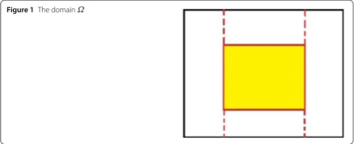
We assume the functionλconstant on eachΩi, 1≤i≤I. We remark that, for any 1≤i≤I, there exists 1≤j≤I, such thatΩi⊂ΩjandI>I. In order to illustrate the decomposi-tion, we consider for exampleI= 2, which means thatΩis built with two heterogeneous regions (see Fig.1). In order to decompose the domain by spectral method, five rectangles (I= 5) are necessary. However, nine rectangles are needed for a conforming decomposi-tion (this means that if the intersecdecomposi-tion of two rectanglesΩiandΩj,i=j, is not empty, it is necessarily equal to a corner or to a hole edge ofΩiandΩj).

We presume that the intersection of each boundary∂Ωi of the sub-domainΩi with the boundary∂Ω of the domainΩis a corner or a hole edge ofΩi. The skeleton of the

decomposition

S= I

i=1

∂Ωi\∂Ω

is equal to: For an integerM≥2

S=

M

m=1

γm, γm∩γm=∅, 1≤m=m≤M, (13)

whereγmstands for mortar. It corresponds to a hole edge of one sub-domainΩinamed Ωi(m).

We considerPNi(Ωi),Ni≥2, 1≤i≤I, the space of the polynomial functions defined on

Ωi, with a degree less or equal toNi, forxandy.

We define the discrete spaceXδ, (δ= (N1, . . . ,NI) is the discrete parameter) as the space of discrete functionsϕδsuch that (see [8]):

• ϕδ_/Ωi,1≤i≤I, belongs to the polynomial spacePNi(Ωi),

• ϕδvanishes on the boundary∂Ω,

• letφthe mortar function whereφ/γm=ϕδ/Ωi(m)/γm, for anyΩi,1≤i≤Iand an edgeΓ

ofΩi(Γ is not part of the boundary∂Ω), we propose the matching condition:

∀χδ∈PNi–2(Γ),

Γ

(ϕδ_/Ωi–φ)(ξ)χδ(ξ)dξ= 0, (14)

wherePNi–2(Γ) is the space of polynomials with degree≤(Ni– 2) defined onΓ. ThatΓ

is not a mortar permits one to conclude that the discretization is not conforming (Xδ is not a subspace ofH1_(Ω)).

For the numerical integration, we use the Gauss–Lobatto quadrature formula on ]–1, 1[. For an integerN≥2, there exists a unique set of pointsε0= –1,εN= 1,εj, 1≤j≤(N– 1) and weightsj, 0≤j≤N, such that

∀ϕ∈P2N–1

]–1, 1[, 1

–1

ϕ(ξ)dξ= N

j=1

ϕ(εj)j. (15)

We deduce the values of the points and weightsε_ijxandx_ij(respectivelyε_ijyandy_ij) in the directionx(respectively in the directiony) fromεj, 0≤j≤Nand weightsj, 0≤j≤N, by homothety and translation of the domainΩito the reference domain ]–1, 1[2. Then we obtain the discrete scalar product: Forϕandψcontinuous on eachΩi, 1≤i≤I,

(ϕ,ψ)δ= I

i=1

(ϕ,ψ)Ni, (16)

where

(ϕ,ψ)Ni=

Ni

j=0

Ni

l=0

We define the space

Zδ=

θδ∈L2(Ω);θδ/Ωi∈PNi(Ωi); 1≤i≤I

,

and Iδthe Lagrange interpolation operator: for allθ∈Xδ such thatθ/Ωi, 1≤i≤Iis

con-tinuous onΩi, Iδ(θ)∈Zδ, and Iδ(θ)(εx_ij,εy_il) =θ(εx_ij,εy_il). Letfn_{be continuous onΩ}

i, 1≤i≤I, for each 0≤n≤M. Consider the discrete problem: Findϕn_δ ∈Xδfor each 1≤n≤M, such that

ϕ_δ0= Iδ(ϕ0)

and

∀ψδ∈Xδ, anδ

ϕ_δn,ψδ=Lnδ(ψδ). (17)

The bilinear forman

δ(·,·), and the linear formLδn(·), for 1≤n≤M, are defined as

anδ

ϕn_δ,ψδ

=ϕn_δ,ψδ

δ+h I

i=1 λi

∇ϕ_δn,∇ψδ

Ni (18)

and

Lnδ(ψδ) =

ϕ_δn–1,ψδ_δ+hfn,ψδ_δ. (19)

We define on the spaceXδthe following broken energy norm:

ψδXδ=

ψδ2_0,Ω+h I

i=1

λi|ψδ|21,Ωi

1 2

. (20)

The bilinear forman

δ(·,·) is continuous onXδ×Xδ, coercive onXδ and the linear form

Lnδ(·) is continuous onXδ. The Lax–Milgram lemma permits us to propose the following theorem.

Theorem 1 For f continuous onΩ×[0,T]andϕ0continuous onΩ,problem(17)has a

unique solution(ϕ_δn)0≤n≤MinYδ×(Xδ)Mverifying the stability condition:

ϕ_δn2_0,Ω+h

n

j=1

I

i=1

λi∇ϕδj0,Ωi≤c

Iδϕ020,Ω+ λmax λmin

n

j=1 _Iδfj

0,Ω

where c is a positive constant independent of n andδ.

3.3 The error estimate

Theorem 2 We supposeλ is constant on each Ωi, 1≤i≤I. Let f is such that f/Ωi ∈ C0_(0,T;Hσi_(Ω

i));σi> 1;ϕ0is such thatϕ0/Ωi∈H

μi_(Ω

i);μi> 1and the solution(ϕn)0≤n≤M

of problem(8)is such thatϕn

/Ωi∈H

si+1_(Ω

i);si≥0.Then the error between the(ϕn)0≤n≤M

and(ϕn_δ)0≤n≤Msolutions of problem(17)is

ϕn_–ϕn δ_n≤ch

(1 +α+αδ)

λmin λmax

I

i=1

λiNi–2silog(Ni)ϕn

2

Hsi+1(Ωi)

1/2

+

1

min(1,λmin₎

1/2I

i=1

N–2σi

i f2_C0_(0,T;Hσi(Ωi))

1/2

+ _I

i=1

N–2μi

i Iδϕ02Hμi(Ωi)

1/2

, (21)

where c is a positive constant independent ofδ,

α= max

1≤m≤M max

k∈η(m)

λk λi(m)

1/2 ,

αδ= max

1≤m≤M max

k∈η(m)

λkNi(m) λi(m)Nk

1/2 .

Remark1 The termαδ vanishes when the decomposition is conforming. The choice of mortars can be done freely in two ways. Firstly, it can be such that

∀k∈η(m), λk≤λi(m). (22)

Thusα≤1.

Secondly, it can be such that

∀k∈η(m), λkNk–1≤λi(m)Ni–1(m), (23)

which can lead us to make a small modification in the domain decomposition. Thus we optimize the error estimation (21) without making the geometry conform.

4 Implementation and numerical results

We start by the description of the implementation of mortar spectral element method for the discrete problem (17). We considerlx_illy_ik, 0≤l,k≤Ni, 1≤i≤I, to be a basis of the polynomial spacePNi(Ωi) wherelxilandl

y

ikdenote the Lagrange interpolating polynomials associated with the nodesεx_ilandε_iky, respectively. Then the solutionϕ_δnof the problem (17) is decomposed as

ϕ_δn(x,y)/Ωi=

Ni l=0 Ni k=0

ϕ_δnε_ilx,ε_ikylx_il(x)ly_ik(y).

Then the discrete problem (17) is written in the form

where Φ_δnis the vector of admissible unknowns composed ofϕ_δn(εx_il,εy_ik), 1≤l,k≤Ni, 1≤i≤I, the matrixDis diagonal with coefficientρ_irxρ_isy, 1≤r,s≤Ni, 1≤i≤I, A is a symmetric block-diagonal matrix made of theIsquare sub-matrices (∇(lillik),∇(lirlis))Ni

which represent the Neumann–Laplace operator on each sub-domainΩi andFnis the vector with components equal to (ϕ_δn–1(εx_ir,ε_isy) +hfn_(εx

ir,ε y is))ρirxρ

y

is, 1≤r,s≤Ni, 1≤i≤I. The vectorΦ_δnhas false degrees of freedom. These false degrees of freedom are the values of the solutionϕ_δnon the edges of the sub-domainΩiwhich are not mortars (Ωi= Ωi(m)) and are not in the boundary∂Ω. Then the matching condition (14) is written in the formϕ_δn_/Γ =Q¯ψ/γm, whereQ¯ is the matching matrix. Its value is determined locally

for each pair edge-mortar (Γ,γm) andψ is the corresponding mortar function (see [15,

16] for more details). Then the action of the global matching matrixQis represented as follows:

vi_lk/internal

vi_lk/edges

Φ_δn =

I 0

0 Q¯

Q

vi_lk/internal ψ/γm

¯

Φ_δn ,

for 1≤i≤I, 1≤l,k≤Niand 1≤m≤M. The role of the matrixQis to decouple the system (24) in order to be solved on each sub-domainΩi. The transpose matrixQTserves to eliminate the false degrees of freedom from the vector of unknowns. Thus the system that we solve is

QT(D+hA)QΦ¯_δn=QTFn. (25)

The components of the vectorΦ¯_δnare the values of the solution on the internal nodes of sub-domainsΩi, 1≤i≤I, and the values of the mortar functions on the skeleton S. Since the matrixA¯=QT_{(D+hA)Qis symmetric and positive defined, we solve the system (25)} using the gradient conjugate method as follows.

Initialization: letΦ₀nbe arbitrary,Rn₀=QT_Fn_–A¯_Φn

0,T0n=Rn0. Iterationk= 1, . . . :

αk= (Rn

k,Rnk) (T_kn,AT¯ _kn),

Φ_kn₊₁=Φ_kn+αkTkn,

Rn_k+1=Rn_k–αkAT¯ kn,

βk=

(Rn_k+1,Rn_k+1) (Rn_k,Rn_k) ,

T_kn₊₁=Rn_k+1+βkTkn.

The high cost of operations is due to the product matrix-vector (D+hA)iΦin, 1≤i≤I, which is of orderO(N4

i). Thanks to the tensorization property of the polynomial basis, this cost has been reduced toO(N3

i) operations.

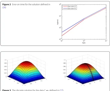
To validate the used numerical method, we focus, firstly, on the time convergence. We consider the domainΩ= ]–1, 1[2_{and the continuous solution}

Figure 2Error on time for the solution defined in (26)

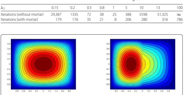
Figure 3The discrete solution for the dataf,ϕ0defined in (27)

We consider the space discrete parameterδ= 40,T= 1 and the time stepsh∈ {10–1_{, 10}–2_, 10–3_{}. Figure2shows the curves of convergence for the two termslogϕ–ϕ}n

δH1_(Ω)(in blue) andlogϕ–ϕn_δL2_(Ω)(in red) as a function oflog(h). We notice that the error de-creases when the stephdecreases with an order almost equal to 1.

In the following, we fixh= 10–3_{,T= 1,}

f(x,y,t) = 1 and ϕ0(x,y) = 0. (27)

We consider the partition of the domainΩ= ]–1, 1[2_{in two sub-domains}

Ω1= ]–1, 0[×]–1, 1[, Ω2= ]0, 1[×]–1, 1[.

Letλ=λ1inΩ1andλ=λ2inΩ2.

In Fig.3(left), the discrete solution is computed forδ=N= 40 without considering the decomposition of the domain whereλis continuous and equal to 1. The discrete solution computed considering the mortar method forδ= (N1,N2) = (40, 40) and (λ1,λ2) = (1, 1) is presented in Fig.3(right).

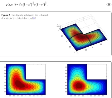
Table 1 Correlation between the number of iterations and the quotientλmax

λmin

λ2 0.15 0.2 0.5 0.8 1 5 10 13 100

Iterations (without mortar) 29,387 1335 72 38 25 388 5598 51,325 ∞ Iterations (with mortar) 179 176 35 21 8 206 280 316 786

Figure 4The isovalues of the discrete solution issued from (27) for (λ1,λ2) = (1, 1) (left) and (λ1,λ2) = (1, 10)

(right)

Figure 5The error curves issued from the solution defined in (26)

In Fig.4, we observe that the discontinuity ofλmakes the discrete solution unsymmet-rical.

To illustrate the variation of the error according to the discontinuity ofλwe define the term:

error=ϕ–ϕ_δn_L2_(Ω) and N=

_I

1

N_i2

1 2 .

Hereafter the error curves showing thelog(error) as a function oflog(N).

In Fig.5(left), the resolution is done without considering the domain decomposition (without mortar) by fixingλ1= 1. The curves are made with a discretization parameter δ∈ {7, 10, 15, 25}. We observe that in the case whereλ2= 1 (in red) and the domain is

However, in Fig.5(right), the same resolution is made considering that the domainΩ is broken down into two sub-domainsΩ1andΩ2. The mortar is chosenγ1= ]–1, 1[ edge ofΩ2,δ equal to (5, 7), (8, 12), (10, 15) and (22, 25). The method is functionally noncon-forming. The curves are made for three different values:λ2= 1 (in red),λ2= 10 (in black) andλ2= 100 (in blue). We observe that in the case whereλ2= 10 andλ2= 100 whereλis discontinuous, the convergence is much better than in the case without domain decom-position. This convergence also depends on the ratio λ2

λ1. Secondly we consider the L-shaped domain

Ω= ]–1, 1[2/ ]0, 1[2,

which we decompose into three sub-domains

Ω1= ]–1, 0[×]–1, 0[, Ω2= ]–1, 0[×]0, 1[, Ω3= ]0, 1[×]–1, 0[.

Figure6presents the discrete solution in the L-shaped domain forδ= (N1,N2,N3) = (35, 35, 35), in the case where the domainΩis homogeneous (i.e.λis continuous equal to (λ1,λ2,λ3) = (1, 1, 1) whereλjis the value ofλon each sub-domainΩjfor 1≤j≤3).

In Fig.7, we present the isovalues of the discrete solution issued from the data (27), for the two valuesλ= (1, 1, 1) andλ= (1, 10, 10). We observe that the symmetry of the solution changes whenλis discontinuous.

Consider the continuous solution

ϕ(x,y,t) =t2x1 –x2

5

2_{y1 –y}252_{. (28)}

Figure 6The discrete solution in the L-shaped domain for the data defined in (27)

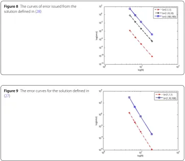
Figure 8The curves of error issued from the solution defined in (28)

Figure 9The error curves for the solution defined in (27)

We choose the two mortarsγ1= ]–1, 0[ inΩ2andγ2= ]–1, 0[ in the sub-domainΩ3. Figure8presents the error curves forλ= (1, 1, 1) (in red),λ= (1, 10, 10) (in black) and λ= (1, 100, 100) (in blue). Each curve is done with a discrete parameterδ= (5, 8, 8),δ= (10, 13, 13),δ= (15, 17, 17) andδ= (20, 25, 25). We notice that in so far as the value of λmax

λmin is high, the error is bad. We also observe that in this case, the error is not as good as in the case of two domains. This is due to the presence of the geometric singularity 3₂π.

Finally, we consider the case of a geometrically nonconforming domain. LetΩ be the domain

Ω= ]–1, 1[2,

partitioned into three sub-domain as follows:

Ω1= ]–1, 1[×]0, 1[, Ω2= ]–1, 0[×]–1, 0[, Ω3= ]0, 1[×]–1, 0[.

5 Conclusion

We have been interested in this work in the numerical implementation of the mortar spec-tral element method for the heat equation with diffusion coefficient depending on the heterogeneity of the domain. We illustrate numerically that the error is poor, which is due to the fact that the diffusion coefficient is piecewise continuous. To improve the order of convergence, we opted for a domain decomposition method (mortar method) associated with the spectral discretization method, known for its high accuracy. This technique can be generalized for other types of partial differential equations.

Acknowledgements

The authors would like to extend their sincere appreciation to the Deanship of Scientific Research at King Saud University for funding this Research group No (RG-1435-026).

Funding Not applicable.

Availability of data and materials Not applicable.

Competing interests

The authors declare that they have no competing interests.

Authors’ contributions

The authors declare that the study was realized in collaboration with equal responsibility. All authors read and approved the final manuscript.

Publisher’s Note

Springer Nature remains neutral with regard to jurisdictional claims in published maps and institutional affiliations.

Received: 12 March 2019 Accepted: 11 April 2019 References

1. Thomée, V.: Galerkin Finite Element Methods for Parabolic Problems. Springer, Paris (1997)

2. Bergam, A., Bernardi, C., Mghazli, Z.: A posteriori analysis of the finite element discretization of some parabolic equations. Math. Compet.251, 1117–1138 (2005)

3. Chorfi, N., Abdelwahed, M., Ben Omrane, I.: A posteriori analysis of the spectral element discretization of heat equation. An. ¸Stiin¸t. Univ. ‘Ovidius’ Constan¸ta22, 13–35 (2014)

4. Zhou, C.: Steady compressible heat-conductive fluid with inflow boundary condition. Bound. Value Probl.2017, 177 (2017)

5. Bernardi, C., Maday, Y.: Adaptive finite element methods for elliptic equations with non-smooth coefficients. Math. Models Methods Appl. Sci.85, 579–608 (2000)

6. Bernardi, C., Chorfi, N.: Mortar spectral element methods for elliptic equations with discontinuous coefficients. Math. Models Methods Appl. Sci.4, 497–524 (2002)

7. Abdelwahed, M., Al Salam, A., Chorfi, N.: Solving the singular two-dimensional fourth order problem by the mortar spectral element method. Bound. Value Probl.2018, 39 (2018)

8. Bernardi, C., Maday, Y., Patera, A.T.: A new nonconforming approch to domain decomposition: the mortar element method. In: Brézis, H., Lions, J.L. (eds.) Nonlinear Partial Differential Equations and Their Applications, pp. 16–27 (1991) Collège de France Seminar

9. Meyers, N.G.: Anlp_{-estimate for the gradient of solutions of second order elliptic divergence equations. Ann. Sc.}

Norm. Super. Pisa17, 189–206 (1963)

10. Chipot, M.: On some stationary Navier–Stokes type problems. Nonlinear Anal., Theory Methods Appl.177, 288–298 (2018)

11. Wohlmuth, B.I.: Discretisation Methods and Iterative Solvers Based on Domain Decomposition. Lecture Notes in Computational Science and Engineering, vol. 17. Springer, Berlin (2001)

12. Seshaiyer, P., Suri, M.: hp submeshing via non-conforming finite element methods. Comput. Methods Appl. Mech. Eng.189, 1011–1030 (2000)

13. Lions, J.L., Magenes, M.: Problèmes aux Limites Non Homogène et Applications. Dunod, Paris (1968)

14. Abdelwahed, M., Chorfi, N.: Mortar spectral elements discretization of the heat equation in an inhomogeneous medium. Comput. Math. Appl. (Submited)

15. Anagnostou, G.: Non conforming sliding spectral element methods for unsteady incompressible Navier–Stokes equation. PhD thesis, Maassachusets Institute of Technology, Cambridge (1991)