SOME NOTES ON THE FAST ADAPTIVE NEURAL NETWORK SOLVERS.

(1)

[Iliev* 4(10): October, 2017] ISSN 2349-4506

Impact Factor: 2.785

G

lobal

J

ournal of

E

ngineering

S

cience and

R

esearch

M

anagement

SOME NOTES ON THE FAST ADAPTIVE NEURAL NETWORK SOLVERS

Anna Malinova, Angel Golev, Anton Iliev*, Nikolay Kyurkchiev

*Faculty of Mathematics and Informatics, University of Plovdiv Paisii Hilendarski, 24, Tzar Asen Str., 4000 Plovdiv, Bulgaria

Faculty of Mathematics and Informatics, University of Plovdiv Paisii Hilendarski, 24, Tzar Asen Str., 4000 Plovdiv, Bulgaria

DOI: 10.5281/zenodo.1034497

KEYWORDS

:

solving polynomial systems of equations, Weierstrass method, non-attractive set of initial approximations.

ABSTRACT

With this paper, we discuss some important aspects related to the iterative solution of two classes of polynomials, nonlinear systems of equations, and the adapted to them – "FAST adaptive neural solver" (FANS). The crucial issue of choosing initial approximations (separation of unattractive networks of initial data) and the possibility of minimizing CPU–time with the use of existing FANS is discussed.

INTRODUCTION

Polynomial systems of equations are of major interest and they are heavily used in any discipline of sciences such as mathematics, physics, chemistry and engineering.

According to [1], [2], the approaches for solving polynomial systems of equations can be classified in two categories as follows:

”1. Symbolic methods that stem from algebraic geometry;

2. Numerical methods, based on iterative procedures. These methods are suitable for local analysis only and perform well only if the initial guess is good enough, a condition that generally is rather difficult to satisfy.” In [1] the authors considered the neural network architecture for the system of polynomials

𝑓𝑖(𝑥) = ∑𝑘𝑗=1𝑖 (𝑎𝑖𝑗∏𝑛𝑙=1𝑥𝑙 𝑒_𝑙𝑗𝑖

) − 𝛽𝑖= 0; 𝑖 = 1,2, … , 𝑛, (1)

where in every exponent 𝑒𝑖_{the superscript}_𝑖_{denotes the equation, the first subscript}_𝑗_{denotes the factor of the} summation in equation 𝑖 and the second subscript 𝑙 denotes the corresponding unknown 𝑥.

Introduced in [1] neural solvers gave good results for polynomial systems associated with chemical engineering applications.

For other results, see [4]–[9].

The point 𝑥̃ ∈ 𝑅𝑛_{is an equilibrium point for the differential equation} 𝑑𝑥

𝑑𝑡 = 𝑔(𝑡, 𝑥) if 𝑔(𝑡, 𝑥̃) = 0 for all 𝑡.

Of course, as we have already mentioned, it remains of crucial importance to choose initial approximations for which researched numerical method or iterative procedure is convergent.

The article is structured as follows. Firstly in “MAIN RESULTS” we explore one special class of polynomial systems and give an analytical description of the non-attractive sets to be considered by the specialists working in the direction - generating of FANS.

(2)

[Iliev* 4(10): October, 2017] ISSN 2349-4506

Impact Factor: 2.785

G

lobal

J

ournal of

E

ngineering

S

cience and

R

esearch

M

anagement

http: // www.gjesrm.com © Global Journal of Engineering Science and Research Management

(appearing as modification of classical Newton-Broyden method).

MAIN RESULTS

We will illustrate the said for a special class of polynomial systems.

Many problems in mathematics and other natural sciences and techniques reduce themselves to determining all roots of a system of equations:

| |

𝑓₁(𝑥) = 𝑥𝑑1_{+ 𝑎}

1,1𝑥𝑑1−1+ ⋯ + 𝑎1,𝑑1= 0, 𝑓2(𝑥) = 𝑥𝑑2+ 𝑎2,1𝑥𝑑2−1+ ⋯ + 𝑎2,𝑑2 = 0, ⋯

𝑓_𝑛(𝑥) = 𝑥𝑑𝑛_{+ 𝑎}

𝑛,1𝑥𝑑𝑛−1+ ⋯ + 𝑎𝑛,𝑑𝑛 = 0,

(2)

where 𝑓_𝑗(𝑥) are polynomials of degree 𝑑_𝑗, 1 ≤ 𝑗 ≤ 𝑛 with simple zeros. Let 𝑥_𝑖,𝑗𝑘_{, 𝑖 = 1,2, … , 𝑛; 𝑗 = 1,2, … , 𝑑} 𝑖, be distinct reasonably close approximations of these zeros. Usually, the Weierstrass procedure is used to solve the problem [45]:

𝑥_𝑖,𝑗𝑘+1= 𝑥_𝑖,𝑗𝑘 − 𝑓𝑖(𝑥𝑖,𝑗 𝑘₎

∏𝑑𝑖_𝑙≠𝑠(𝑥𝑖,𝑙𝑘−𝑥𝑖,𝑠𝑘)

; 𝑗 = 1,2, … , 𝑑𝑖; 𝑖 = 1,2, … , 𝑛.

Finding the zeros of the polynomial system (2) is related closely to research in the area of ”chemical equilibrium applications”, ”kinematic applications” and others. Following the ideas given in [34], [30] we obtain

∑𝑑𝑟

𝑝=1 𝑥𝑟,𝑝𝑘+1= −𝑎𝑟,1, ∑𝑑𝑟

𝑝=1 𝑥𝑟,𝑝𝑘+1∑𝑑𝑞≠𝑝𝑟 𝑥𝑟,𝑞𝑘 = ∑𝑙<𝑠𝑑𝑟 𝑥𝑟,𝑙𝑘 𝑥𝑟,𝑠𝑘 + 𝑎𝑟,2, ∑𝑑𝑟

𝑝=1 𝑥𝑟,𝑝𝑘+1∑𝑙<𝑠;𝑙,𝑠≠𝑝𝑥𝑟,𝑙𝑘𝑥𝑟,𝑠𝑘 = 2 ∑𝑙<𝑠<𝑡𝑑𝑟 𝑥𝑟,𝑙𝑘 𝑥𝑟,𝑠𝑘 𝑥𝑟,𝑡𝑘 − 𝑎𝑟,3, …

∑𝑑𝑟

𝑝=1 𝑥𝑟,𝑝𝑘+1∏𝑑𝑞≠𝑝𝑟 𝑥𝑟,𝑞𝑘 = (𝑑𝑟− 1) ∏𝑑𝑞=1𝑟 𝑥𝑟,𝑞𝑘 + (−1)𝑑𝑟𝑎𝑟,𝑑𝑟, ; 𝑟 = 1,2, … , 𝑛.

(3)

The resulting systems of equations (3) can be written in vector form as: 𝐴𝑟_𝑑_𝑟_𝑥

𝑟𝑑𝑟 𝑘+1_{= 𝑏}

𝑑𝑟

𝑟 _{; 𝑟 = 1,2, … , 𝑛,}

where

𝐴_𝑑𝑟_𝑟_{: =}

(

1 1 … 1

∑_𝑞≠1𝑥_𝑟,𝑞𝑘 _∑

𝑞≠2 𝑥𝑟,𝑞𝑘 … ∑𝑞≠𝑑𝑟 𝑥𝑟,𝑞 𝑘

⋮ ⋮ ⋮

∏_𝑞≠1𝑥_𝑟,𝑞𝑘 _∏

𝑞≠2𝑥𝑟,𝑞𝑘 … ∏𝑞≠𝑑𝑟 𝑥𝑟,𝑞𝑘 ) ,

𝑑𝑒𝑡𝐴_𝑑𝑟_𝑟_{= ∏}𝑑𝑟

𝑖<𝑗(𝑥𝑟,𝑖𝑘 − 𝑥𝑟,𝑗𝑘 ) ≠ 0,

𝑥_𝑟𝑑𝑘+1_𝑟_{: =}

( 𝑥_𝑟,1𝑘+1 𝑥_𝑟,2𝑘+1 ⋮ 𝑥_𝑟,𝑑𝑘+1_𝑟

) ,

𝑏_𝑑𝑟_𝑟_{: =}

( 𝑏_𝑟,1𝑑𝑟

𝑏_𝑟,2𝑑𝑟 ⋮ 𝑏_𝑟,𝑑𝑑𝑟_𝑟 ) = ( −𝑎_𝑟,1 ∑𝑑𝑟

𝑙<𝑠 𝑥𝑟,𝑙𝑘𝑥𝑟,𝑠𝑘 + 𝑎𝑟,2 ⋮

(𝑑_𝑟− 1) ∏𝑑𝑟

𝑞=1𝑥𝑟,𝑞𝑘 + (−1)𝑑𝑟𝑎𝑟,𝑑𝑟₎

, 𝑟 = 1,2, … , 𝑛.

We shall use also the notations 𝑆_𝑚𝑟,𝑑𝑟_{: = ∑}

1≤𝑖1<𝑖2<⋯<𝑖𝑚≤𝑑𝑟 𝑥𝑟,𝑖1 𝑘 _{… 𝑥}

𝑟,𝑖𝑚

(3)

[Iliev* 4(10): October, 2017] ISSN 2349-4506

Impact Factor: 2.785

G

lobal

J

ournal of

E

ngineering

S

cience and

R

esearch

M

anagement

Then

𝑏_𝑟,𝑚𝑑𝑟 _{= (𝑚 − 1)𝑆}

𝑚𝑟,𝑑𝑟+ (−1)𝑚𝑎𝑟,𝑚, 𝑟 = 1,2, … , 𝑛; 𝑚 = 1,2, … , 𝑑𝑟. For any given 1 ≤ 𝑖 < 𝑗 ≤ 𝑑_𝑟, 𝑟 = 1,2, … , 𝑛, we define the polynomials:

𝜔_𝑖𝑗𝑟,𝑑𝑟_{(𝑥) = (𝑥 − 𝑥}

𝑟,1𝑘 ) … (𝑥 − 𝑥𝑟,𝑖−1𝑘 )(𝑥 − 𝑥𝑟,𝑖+1𝑘 ) … (𝑥 − 𝑥𝑟,𝑗−1𝑘 )(𝑥 − 𝑥𝑟,𝑗+1𝑘 ) … (𝑥 − 𝑥𝑟,𝑑𝑟 𝑘 _).

We have the following theorem.

Theorem A. [37] Suppose that for some 1 ≤ 𝑖 < 𝑗 ≤ 𝑑𝑟, 𝑟 = 1,2, … 𝑛, the sequence of approximations 𝑥_𝑟,1𝑘 _{, … , 𝑥}

𝑟,𝑑𝑟

𝑘 _,_{𝑟 = 1,2, … , 𝑛,}_{satisfies the conditions}

∑𝑑𝑟

𝑚=1(−1)𝑚𝑏𝑟,𝑚𝑑𝑟 [𝜔𝑖𝑗 𝑟,𝑑𝑟_(𝑥

𝑟,𝑗𝑘 )(𝑥𝑟,𝑖𝑘 ) 𝑑𝑟−𝑚

+ 𝜔_𝑖𝑗𝑟,𝑑𝑟_(𝑥 𝑟,𝑖 𝑘 _)(𝑥

𝑟,𝑗𝑘 ) 𝑑𝑟−𝑚

] = 0, (4)

𝑟 = 1,2, … , 𝑛. Then 𝑥_𝑟,𝑖𝑘+1_{= 𝑥}

𝑟,𝑗𝑘+1, 𝑟 = 1,2, … , 𝑛, and thus, the (k+2)-th step of the Weierstrass method cannot be performed.

The set 𝐷_𝑓[𝑓₁_,…,𝑓_𝑛_] of the non-attractive starting points is the set of points satisfying equations (4).

Example 1. We consider the system (Mamat et al. [3], Goulianis et al. [1]): 𝑓_𝑖(𝑥) = 𝑥_𝑖2_{+ 𝑥}

𝑖− 2 = 0, 𝑖 = 1,2, … , 𝑛. (5)

Let 𝑛 = 2. The non-attractive set 𝐷𝑓[𝑓1,𝑓2] is given by (see, (4)) 𝐷_𝑓[𝑓₁_,𝑓₂_]= ⋃2

𝑖=1 𝐷𝑓𝑖, where

𝐷𝑓1: 2𝑥1,1 𝑘 _𝑥

1,2𝑘 + 𝑥1,1𝑘 + 𝑥1,2𝑘 − 4 = 0, 𝐷𝑓2: 2𝑥2,1𝑘 𝑥2,2𝑘 + 𝑥2,1𝑘 + 𝑥2,2𝑘 − 4 = 0.

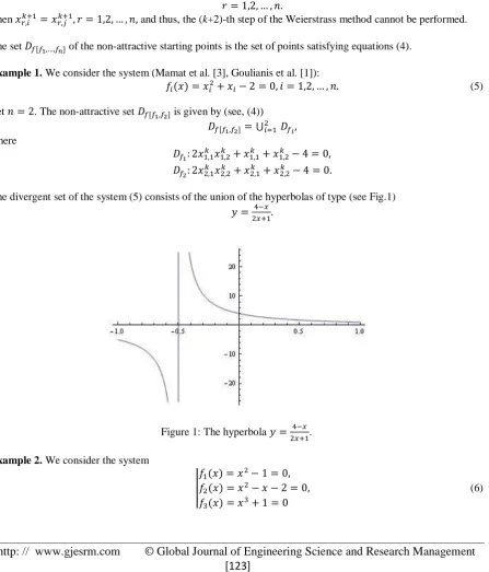
The divergent set of the system (5) consists of the union of the hyperbolas of type (see Fig.1) 𝑦 = 4−𝑥

2𝑥+1.

Figure 1: The hyperbola 𝑦 = 4−𝑥 2𝑥+1.

Example 2. We consider the system

|

𝑓1(𝑥) = 𝑥2− 1 = 0, 𝑓2(𝑥) = 𝑥2− 𝑥 − 2 = 0, 𝑓₃(𝑥) = 𝑥3_{+ 1 = 0}

(4)

[Iliev* 4(10): October, 2017] ISSN 2349-4506

Impact Factor: 2.785

G

lobal

J

ournal of

E

ngineering

S

cience and

R

esearch

M

anagement

which has root −1. The non-attractive set 𝐷𝑓[𝑓1,𝑓2,𝑓3] is given by (see, (4)) 𝐷𝑓[𝑓1,𝑓2,𝑓3]= ⋃

3 𝑖=1𝐷𝑓𝑖, where

𝐷𝑓1: 𝑥1,1 𝑘 _𝑥

1,2𝑘 − 1 = 0, 𝐷_𝑓₂: 𝑥_2,2𝑘 _(2𝑥

2,1𝑘 − 1) = 4 + 𝑥2,1𝑘 , 𝐷_𝑓₃: (𝑥_3,1𝑘 _{− 𝑥}

3,2𝑘 )2(𝑥3,3𝑘 )2+ (2 + 𝑥3,1𝑘 (𝑥3,2𝑘 )2+ (𝑥3,1𝑘 )2𝑥3,2𝑘 )𝑥3,3𝑘 −(2(𝑥_3,1𝑘 ₎2_(𝑥

3,2𝑘 )2+ 𝑥3,1𝑘 + 𝑥3,2𝑘 ) = 0.

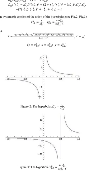
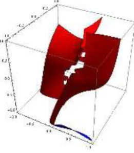
The divergent set of the system (6) consists of the union of the hyperbolas (see Fig.2–Fig.3)

𝑥_1,2𝑘 ₌ 1 𝑥1,1𝑘 , 𝑥2,2

𝑘 ₌ 4+𝑥2,1𝑘 2𝑥2,1𝑘 −1

and surface (see Fig. 4).

𝑧 =−(2+𝑥𝑦2+𝑥2𝑦)+𝜀√(2+𝑥𝑦2+𝑥2𝑦)2+4(𝑥−𝑦)2(2𝑥2𝑦2+𝑥+𝑦)

2(𝑥−𝑦)2 , 𝜀 = ±1,

(𝑧 = 𝑥_3,3𝑘 _{; 𝑥 = 𝑥}

3,1𝑘 ; 𝑦 = 𝑥3,2𝑘 ).

Figure 2: The hyperbola 𝑥_1,2𝑘 ₌ 1 𝑥1,1𝑘 .

(5)

[Iliev* 4(10): October, 2017] ISSN 2349-4506

Impact Factor: 2.785

G

lobal

J

ournal of

E

ngineering

S

cience and

R

esearch

M

anagement

Figure 4: The surface 𝑧.

Remarks

In the Example 1, the Newton’s procedure does not converge for 𝑛 > 2 and Weierstrass procedure fails for the non-attractive set 𝐷_𝑓[𝑓₁_,𝑓₂_] of initial approximations.

The Example 2 is very instructive and divergent set of initial approximations 𝐷𝑓[𝑓1,𝑓2,𝑓3] is very complicated. In studying the equilibrium state of some classes of differential systems that require the study of polynomial systems of the type (2) it is extremely important to "separate" the non-attractive initial approximations to the roots. For an arbitrary 𝑛 the description of conditions (4) it is not difficult due to the existing symmetry.

You will explicitly note that for all known classic and newer algorithms like Chebishev, Halley, Ehrlich, Abert, Nourein, Dvorchuk, Petkovic, Kyurkchiev, Iliev, Proinov and others(see, [29], [31]–[33], [35]–[36], [38]–[43]) to solve the assigned task are derived and described in details respective non-attractive sets of initial data that are permanently present in the implemented scientific platform (intellectual property, see, for instance [44]). This is a very important element in dealing with issues of the mentioned issues.

First of all, the user of such algorithms usually is naturalist and a priori is not supposed to be a specialist in "Applied Mathematics".

In this sense, the requirements to user of choosing initial approximations by using different subroutines and products included in program environments and platforms are highly restrictive.

Program modules in contemporary environments must be so set to automatically report ”non-attractive sets” (as we have noted - it is not difficult their description) and to provide the user reliable solution to the problem. Goulianis et al. [1] showed that the proposed adaptive neural network algorithm is characterized by fast convergence for high–dimensional systems.

Of course analogous questions regarding the appropriate choice of initial approximations can be found in the existing and described in the literature adaptive neural network solvers.

Inevitably that will mean – ”better CPU–time”.

Solving the more general polynomial systems class of the type (1)

General iteration process, which possesses order of convergence 𝑡 is constructed in [32], [33]. From this process, Newton’s iteration formula (𝑡 = 2) and Halley’s iteration formula (𝑡 = 3) are received as particular cases. The used technique is based on generalized Taylor’s formula.

Let the system of equations

𝑓_𝑖(𝑥⃗_𝑘) = 0, 𝑖 = 1,2, . . . , 𝑛 (7) be given.

Supposed that 𝑓_𝑖 and the partial derivatives of these functions of sufficiently high order are continuous in the neighborhood of solution 𝜉⃗(𝜉1, 𝜉2, . . . , 𝜉𝑛).

(6)

[Iliev* 4(10): October, 2017] ISSN 2349-4506

Impact Factor: 2.785

G

lobal

J

ournal of

E

ngineering

S

cience and

R

esearch

M

anagement

degree 𝑡 − 1 with respect of ℎ𝑠_{will be included. Taylor’s formula is of the form} 0 = 𝑓𝑖+ 𝑓𝑖𝑖1

(1) ℎ𝑖1₊1

2!𝑓𝑖𝑖1𝑖2 (1)

ℎ𝑖1_ℎ𝑖2₊1 3!𝑓𝑖𝑖1𝑖2𝑖3

(1)

ℎ𝑖1_ℎ𝑖2_ℎ𝑖3

+. . . + 1

(𝑡−1)!𝑓𝑖𝑖1𝑖2...𝑖𝑡−1 (1)

ℎ𝑖1_ℎ𝑖2_{. . . ℎ}𝑖𝑡−1_{+ 𝑂̅(𝜀}𝑡_). (8)

Following the scheme by which Newton’s and Halley’s iteration formulae were developed we suppose that in the above consideration we have determined

ℎ𝑗_{= 𝐻} 𝑡−2

𝑗 _{+ 𝑂}𝑗_(𝜀𝑡−1₎ ₍₉₎

and

‖𝑂_𝑖(𝜀𝑡−1_{)‖ ≤ 𝑀}

𝑡−1∗ 𝜀𝑡−1. (10)

Then, after replacing ℎ𝑗_{from (10) in (9) we receive} 0 = 𝑓𝑖+ (𝑓𝑖𝑖(1)

1 ₊1 2!𝑓𝑖𝑖1𝑖2

(1)

𝐻_𝑡−1𝑖2 ₊1 3!𝑓𝑖𝑖1𝑖2𝑖3

(1)

𝐻_𝑡−1𝑖2 _𝐻 𝑡−1 𝑖3

+. . . +_(𝑡−1)!1 𝑓_𝑖𝑖(1)₁_𝑖₂_...𝑖_𝑡−1𝐻_𝑡−1𝑖2 _𝐻 𝑡−1 𝑖3 _{. . . 𝐻}

𝑡−1

𝑖𝑡−1_{) ℎ}𝑖1₊1 2!𝑓𝑖𝑖1𝑖2

(1)

𝑂𝑖2_(𝜀𝑡−1_)ℎ𝑖1

+1 3!𝑓𝑖𝑖1𝑖2𝑖3

(1) _(𝑂𝑖2(𝜀𝑡−1)𝐻 𝑡−1

𝑖3 _{+ 𝑂}𝑖3(𝜀𝑡−1)𝐻 𝑡−1

𝑖2 _{+ 𝑂}𝑖2(𝜀𝑡−1)𝑂𝑖3(𝜀𝑡−1)) ℎ𝑖1

+. . . +_(𝑡−1)!1 𝑓_𝑖𝑖(1)₁_𝑖₂_...𝑖_𝑡−1(𝑂𝑖2_(𝜀𝑡−1_)𝐻 𝑡−1

𝑖3 _𝐻 𝑡−1

𝑖4 _{. . . 𝐻} 𝑡−1

𝑖𝑡−1

+. . . +𝐻_𝑡−1𝑖2 _(𝜀𝑡−1_)𝐻 𝑡−1

𝑖3 _(𝜀𝑡−1_{). . . 𝑂}𝑖𝑡−1_(𝜀𝑡−1₎

+𝑂𝑖2_(𝜀𝑡−1_)𝑂𝑖3_(𝜀𝑡−1_{). . . )ℎ}𝑖1_{+ 𝑂̅} 𝑖(𝜀𝑡).

(11)

The system (11) we write in the form

0 = 𝑓_𝑖+ 𝑓_𝑖𝑖 1

(𝑡)_ℎ𝑖1_{+ 𝑂}

𝑖(𝜀𝑡), (12)

where we substitute

𝑓_𝑖𝑖(𝑡)₁ = 𝑓_𝑖𝑖1₁₊1 2!𝑓𝑖𝑖1𝑖2

(1)

𝐻_𝑡−1𝑖2 _{+. . . +} 1

(𝑡−1)!𝑓𝑖𝑖1𝑖2...𝑖𝑡−1

1 _𝐻

𝑡−1 𝑖2 _𝐻

𝑡−1 𝑖3 _{. . . 𝐻}

𝑡−1 𝑖𝑡−1

and

𝑂𝑖(𝜀𝑡) = 1 2!𝑓𝑖𝑖1𝑖2

(1)

𝑂𝑖2_(𝜀𝑡−1_)ℎ𝑖1₊1 3!𝑓𝑖𝑖1𝑖2𝑖3

(1) _(𝑂_𝑖₂

(𝜀𝑡−1_)𝐻 𝑡−1

𝑖3 _{+ 𝑂}𝑖3_(𝜀𝑡−1_)𝐻 𝑡−1 𝑖2

+𝑂𝑖2(𝜀𝑡−1)𝑂𝑖3(𝜀𝑡−1)) ℎ𝑖1_{+. . . +} 1 (𝑡−1)!(𝑂

𝑖2(𝜀𝑡−1)𝐻 𝑡−1 𝑖3 _𝐻

𝑡−1 𝑖4 _{. . . 𝐻}

𝑡−1 𝑖𝑡−1

+. . . +𝐻_𝑡−1𝑖2 _(𝜀𝑡−1_)𝐻 𝑡−1

𝑖3 _(𝜀𝑡−1_{). . . 𝑂}𝑖𝑡−1(𝜀𝑡−1)+. . . )ℎ𝑖1_{+ 𝑂̅} 𝑖(𝜀𝑡).

The elements of reciprocal matrix of {𝑓_𝑖𝑖 1 (𝑡)

} we denote with 𝑓_(𝑡)𝑖𝑖1_{. From the system (12) we determine}_ℎ𝑖1

ℎ𝑖1_{= −𝑓} (𝑡)

𝑖1𝑠_𝑓 𝑠+ 𝑓(𝑡)

𝑖1𝑠_𝑂

𝑠(𝜀𝑡). (13)

We substitute 𝐻_𝑡−1𝑖1 _{= −𝑓} (𝑡)

𝑖1𝑠_𝑓 𝑠.

The following iteration formula can be formed:

𝑥_𝑘+1𝑠 _{= 𝑥}

𝑘𝑠+ 𝐻𝑡−1𝑠 , (14)

where 𝑡 denotes order of convergence. Let us form the expression

𝜉𝑠_{− 𝑥}

(𝑘)𝑠 − 𝐻𝑡𝑠= 𝜉𝑠− 𝑥(𝑘+1)𝑠 = ℎ𝑠− 𝐻𝑡𝑠= 𝑂𝑠(𝜀𝑡). We have

‖𝑂𝑖(𝜀𝑡)‖ ≤ 1 2!‖𝑓𝑖𝑖1𝑖2

(1)_‖‖𝑂_𝑖₂

(𝜀𝑡−1_)‖‖ℎ𝑖1_‖

+1

3!(‖𝑓𝑖𝑖1𝑖2𝑖3 (1) _{‖ ‖𝑂}_𝑖₂

(𝜀𝑡−1_)‖‖ℎ𝑖1_{‖ + ‖𝑓} 𝑖𝑖1𝑖2𝑖3

(1) _{‖ ‖𝑂}_𝑖₃

(7)

[Iliev* 4(10): October, 2017] ISSN 2349-4506

Impact Factor: 2.785

G

lobal

J

ournal of

E

ngineering

S

cience and

R

esearch

M

anagement

+. . . + 1

(𝑡−1)!(‖𝑓𝑖𝑖1𝑖2...𝑖𝑡−1

(1) _{‖ ‖𝑂}𝑖2(𝜀𝑡−1)‖‖𝐻 𝑡−1 𝑖3 _{‖. . . ‖𝐻}

𝑡−1 𝑖𝑡−1_‖

+. . . + ‖𝑓_𝑖𝑖 1𝑖2...𝑖𝑡−1 (1) _{‖ ‖𝐻}

𝑡−1 𝑖2 _‖‖𝐻

𝑡−1

𝑖3 _{‖. . . ‖𝑂}𝑖𝑡−1_(𝜀𝑡−1_{)‖+. . . ) + ‖𝑂̅(𝜀}𝑡_)‖

and

‖𝑂̅𝑖(𝜀𝑡)‖ = ‖𝑓𝑖𝑖1𝑖2...𝑖𝑡 (1)

ℎ𝑖1_ℎ𝑖2_{. . . ℎ}𝑖𝑡_{‖ ≤ ‖𝑓} 𝑖𝑖1𝑖2...𝑖𝑡

(1)

‖ ‖ℎ𝑖1_‖‖ℎ𝑖2_{‖. . . ‖ℎ}𝑖𝑡_{‖ ≤ ‖𝑓} 𝑖𝑖1𝑖2...𝑖𝑡

(1) ‖ 𝜀𝑡_,

where all summands which contained multipliers 𝜀𝑠_{are dropped, when}_{𝑠 > 𝑡}_.

Taking into account the fact that functions 𝑓𝑖 are sufficiently smooth and that in above estimates all summands are of order 𝑂_𝑖(𝜀𝑡₎_.

We conclude that the following upper bound is valid

‖𝑂_𝑖(𝜀𝑡_{)‖ ≤ 𝑀}

𝑡∗𝜀𝑡, (15)

where 𝑀𝑡∗ is a positive constant.

Using (15) we receive the inequalities ‖𝜉𝑠_{− 𝑥}

(𝑘+1)𝑠 ‖ ≤ ‖𝑂𝑠(𝜀𝑡)‖ ≤ 𝑀𝑡∗𝜀𝑡‖𝑓𝑡 𝑖1𝑙_‖.

|

𝑓₁(𝑥) = 0.25𝑥₁2_{+ 𝑥}

22− 1 = 0,

𝑓2(𝑥) = 𝑥12− 2𝑥1+ 𝑥22= 0, (16)

Figure 5: The structure of neural solver for Example 3. [1].

When we apply formula (14) to solve system from Example 3 for 𝑡 = 3 with initial approximations (1; −1), (1; 1) and (3; 1) with accuracy 15 decimal digits the respectively results are

(0.666666666666667; −0.942809041582063),

(0.666666666666667; 0.942809041582063) and

(8)

[Iliev* 4(10): October, 2017] ISSN 2349-4506

Impact Factor: 2.785

G

lobal

J

ournal of

E

ngineering

S

cience and

R

esearch

M

anagement

For specifying the double root (2,0), appropriate modification of the method outlined above is used.

|

𝑓1(𝑥) = 𝑥1𝑥22− 3𝑥13𝑥22− 5 = 0, 𝑓₂(𝑥) = 2𝑥₁3_𝑥

22+ 2𝑥14𝑥24− 4𝑥12𝑥24+ 3 = 0, (17)

Figure 6: The structure of neural solver for Example 4. [1].

We have used the formula (14) for finding solutions of system from Example 4 for 𝑡 = 3 with initial approximations (−1.9; 0.7), (−1.9; −0.7), (−3.6; 0.2) and (−3.6; −0.2) with accuracy 15 decimal digits and the respectively results are

(−1.70807408954102; 0.614482226647498),

(−1.70807408954102; −0.614482226647499),

(−3.32903633273033; 0.215813224817305) and

(−3.32903633273034; −0.215813224817305) for 4 iterations only.

Figure 7: Higher order recurrent neural networks.

(9)

[Iliev* 4(10): October, 2017] ISSN 2349-4506

Impact Factor: 2.785

G

lobal

J

ournal of

E

ngineering

S

cience and

R

esearch

M

anagement

CONCLUDING REMARKS

Part of the notes in “Remarks” remain valid for solving arbitrary systems of nonlinear equations.

Here is also interesting the question of isolating the non-attractive initial approximations using different modifications of the classic Newton–Broyden type methods with high order of convergence 𝑡.

The much broader issue of selecting initial data for solving polynomial systems of type (1) can be considered as open.

Sigmoidal functions (also known as ”activation functions”) find multiple applications to neural networks [10]– [15].

In conclusion, we will note that the newly constructed recurrently generable families of sigmoidal and activation functions (see, for instance [16]–[28]) can be used with success in creating a new higher order recurrent neural networks (Fig. 7).

Of course the specialists working in this important area also have the task of exploring eventual possibility for minimizing CPU–time using the existing and new ones FANS.

ACKNOWLEDGMENTS

This work has been supported by the project FP17–FMI–008 of Department for Scientific Research, Paisii Hilendarski University of Plovdiv.

REFERENCES

1. K. Goulianis, A. Margaris, I. Refandis, K. Diamantaras, Solving polynomial systems using a fast adaptive back propagation–type neural network algorithm, Euro. Jnl of Applied Mathematics, 2017, 1–37. 2. D. Manocha, Solving systems of polynomial equations, IEEE Comput. Graph. Appl., 14 (2), 1994, 46–

55

3. M. Mamat, K. Muhamad, M.Y. Waziri, Trapezoidal Broyden’s method for solving systems of nonlinear equations, Appl. Math. Sci. 8 (6), 2014, 251–260

4. T. Nguyen, Neural network architecture of solving nonlinear equation systems, Electron. Lett., 29 (16), 1993, 1403–1405

5. K. Mathia, R. Saeks, Solving nonlinear equations using recurrent neural networks, In: World Congress on Neural Networks (WCNN’ 95), Washington DC, pp. 76–80

6. X. Guo, Z. Zeng, The neural–network approaches to solve nonlinear equation, J. Comput., 5 (3), 2010, 410–416

7. A. Margaris, M. Adamopoulos, Solving nonlinear algebraic systems using artificial neural networks, In: Proceedings of the 10th international conference of engineering applications of artificial neural networks, Thessaloniki, Greece, 2007

8. N. Hahm, B.I. Hong, A note on neural network approximation with a sigmoidal function, Appl. Math. Sci., 10 (42), 2016, 2075–2085

9. K. Goulianis, A. Margaris, I. Refandis, K. Diamantaras, T. Papadimitriou, A back propagation–type neural network architecture for solving the complete 𝑛 × 𝑛 nonlinear algebraic system of equations, Adv. in Pure Math., 6, 2016, 455–480.

10. D. Costarelli, R. Spigler, Approximation results for neural network operators activated by sigmoidal functions, Neural Networks 44, 101–106 (2013).

11. D. Costarelli, G. Vinti, Pointwise and uniform approximation by multivariate neural network operators of the max-product type, Neural Networks, 2016; doi:10.1016/j.neunet.2016.06.002; http://www.sciencedirect.com/science/article/pii/S0893608016300685.

12. D. Costarelli, R. Spigler, Solving numerically nonlinear systems of balance laws by multivariate sigmoidal functions approximation, Computational and Applied Mathematics 2016; DOI:10.1007/s40314-016-0334-8 http://link.springer.com/article/10.1007/s40314-016-0334-8

13. D. Costarelli, G. Vinti, Convergence for a family of neural network operators in Orlicz spaces, Mathematische Nachrichten 2016; doi:10.1002/mana.20160006

14. N. Gyliyev, V. Ismailov, On the approximation by single hidden layer feed forward neural networks with fixed weights, arXiv:1708.06219v1 [cs. NE] 21 August (2017)

(10)

[Iliev* 4(10): October, 2017] ISSN 2349-4506

Impact Factor: 2.785

G

lobal

J

ournal of

E

ngineering

S

cience and

R

esearch

M

anagement

16. N. Kyurkchiev, A. Iliev, S. Markov, Some techniques for recurrence generating of activation functions, LAP LAMBERT Academic Publishing, 2017; ISBN 978-3-330-33143-3.

17. Malinova, A., A. Golev, A. Iliev, N. Kyurkchiev, A Family of Recurrence Generating Activation Functions Based on Gudermann Function, International Journal of Engineering Researches and Management Studies, 4(8), 2017, 38-48, ISSN: 2394-7659

18. N. Kyurkchiev, A. Iliev, A note on the new Fibonacci hyperbolic tangent activation function, Int. J. of Innovative Science, Engineering and technology, 4 (5), 2017.

19. Golev, A., A. Iliev, N. Kyurkchiev, A Note on the Soboleva’ Modified Hyperbolic Tangent Activation Function, International Journal of Innovative Science Engineering and Technology, 4 (6), 2017. 20. N. Kyurkchiev, S. Markov, Sigmoid functions: Some Approximation and Modelling Aspects. (LAP

LAMBERT Academic Publishing, Saarbrucken, 2015); ISBN 978-3-659-76045-7.

21. V. Kyurkchiev, A. Iliev, N. Kyurkchiev, On some families of recurrence generated activation functions, Int. J. of Sci. Eng. And Appl. Sci., 3 (3), 2017; ISSN:2395-370

22. N. Kyurkchiev, A family of recurrence generated sigmoidal functions based on the Verhulst logistic function. Some approximation and modeling aspects, Biomath Communications, 3 (2), (2016); 18 pp., http://www.biomathforum.org/biomath/index.php/conference/article/view/789/873

23. N. Kyurkchiev, A note on the Volmer’s activation function, Compt. rend. Acad. bulg. Sci., 70 (6), 2017, 769-776

24. A. Iliev, N. Kyurkchiev, S. Markov, A family of recurrence generated parametric activation functions with applications to neural networks, International Journal on Research Innovations in Engineering Science and Technology, 2 (1), 60–68, 2017.

25. N. Kyurkchiev, S. Markov, Hausdorff Approximation of the Sign Function by a Class of Parametric Activation Functions, Biomath Communications, 3 (2), (2016); 14 pp., http://dx.doi.org/10.11145/bmc.2016.12.217

26. N. Kyurkchiev, A. Iliev, S. Markov, Families of recurrence generated three and four parametric activation functions, Int. J. Sci. Res. and Development, 4 (12), 746-750, 2017.

27. V. Kyurkchiev, N. Kyurkchiev, A family of recurrence generated functions based oh Half-hyperbolic tangent activation functions, Biomedical Statistics and Informatics, 2 (3). 87-94, 2017,

28. Iliev, A., N. Kyurkchiev, S. Markov, A Note on the New Activation Function of Gompertz Type, Biomath Communications, 4(2), 2017 (accepted).

29. Petkovic, M., D. Herceg, S. Ilic, Point Estimation Theory and its Applications, Institute of Mathematics, Novi Sad, 1997

30. Hristov V., N. Kyurkchiev, A note on the globally convergent properties of the Weierstrass-Dochev method, Approximation Theory, A volume dedicated to Bl. Sendov (B. Boyanov Ed.), DARBA, Sofia, 2002, 231-240.

31. Kyurkchiev N., Initial approximations and root finding methods, Mathematical Research Vol. 104, Wiley-VCH Verlag Berlin GmbH, Berlin, 1998.

32. Iliev, A., I. Iliev. Numerical method with order t for solving system nonlinear equations, Collection of scientific works, 30 years FMI, Plovdiv, 2000, 105-112.

33. A. Iliev, N. Kyurkchiev, Nontrivial methods in numerical analysis, Selected topics in numerical analysis, LAP LAMBERT Academic Publishing, GmbH Co. KG, Saarbrucken, 2010.

34. Kyurkchiev N., Some remarks on Weierstrass root-finding method, Compt. rend. Acad. bulg. Sci., 46, No 8, 1993, 17–20.

35. Petkovic, M., N. Kyurkchiev, A note on the convergence of the Weierstrass SOR method for polynomial roots, J. Comput. Appl. Math., 80 (1), 1997, 163–168

36. Valchanov, N., A. Golev, A. Iliev, On the critical points of Kyurkchiev’s method for solving algebraic equations, Serdica J. Computing, 9 (1), 2015, 27–34

37. Hristov, V., N. Kyurkchiev, A. Iliev, On the solutions of polynomial systems obtained by Weierstrass method, C. R. Acad. Bulg. Sci., 62, No 11, 2009, 1371–1376

38. P. Proinov, New general convergence theory for iterative processes and its applications to Newton– Kantorovich type theorems, Journal of Complexity 26, 2010, 3–42.

(11)

[Iliev* 4(10): October, 2017] ISSN 2349-4506

Impact Factor: 2.785

G

lobal

J

ournal of

E

ngineering

S

cience and

R

esearch

M

anagement

40. P. Proinov, M. Vasileva, On the convergence of high-order Ehrlich-type iterative methods for approximating all zeros of a polynomial simultaneously, Journal of Inequalities and Applications, 336, 2015, doi:10.1186/s13660-015-0855-5

41. P. Proinov, S. Cholakov, Semilocal convergence of Chebyshev-like root-finding method for simultaneous approximation of polynomial zeros, Applied Mathematics and Computation, 236, 2014, 669-682.

42. P. Proinov, S. Ivanov, On the Convergence of Halley’s Method for Multiple Polynomial Zeros, Mediterranean Journal of Mathematics, 2015, 12(2), 555–572.

43. P. Proinov, M. Petkova, Convergence of the Weierstrass method for simultaneous approximation of polynomial zeros, C. R. Acad. Bulg. Sci., 66(6), 2013, 809-818.

44. Valchanov, N., Modeling and Implementation of Extensible Modular Information Systems, PhD Thesis, University of Plovdiv, Plovdiv, 2012