ISSN: 2374-2348 (Print), 2374-2356 (Online) Copyright © The Author(s).All Rights Reserved. Published by American Research Institute for Policy Development DOI: 10.15640/arms.v4n2a2 URL: https://doi.org/10.15640/arms.v4n2a2
Fourier Series for Functions Defined on Arbitrary Limited Intervals with Polynomial
Expansion
Xianping Li
1Abstract
Fourier series for functions defined on general interval [ , ] are discussed. Polynomial expansions to larger domain are introduced that can achieve the desired smoothness and improve the convergence rate.
Keywords: Fourier series, polynomial expansion, convergence, smoothness, arbitrary interval
1. Introduction
Fourier series are extensively discussed for periodic functions defined on intervals − , or [0, ], where is the period. For aperiodic functions defined on limited intervals, they are usually expanded to a periodic function within the same domain. Half-range sine or cosine expansions are commonly used to expand the function to a larger domain [6, 2, 4]. However, half-range sine or cosine expansions may lead to discontinuous or non-differentiable periodic functions and the corresponding Fourier series converges slowly.
Polynomial interpolation methods have been developed to accelerate the convergence of the Fourier series [3, 1]. The original function is modified by a system of Lanczos polynomials to achieve a desired smoothness. Alternative forms of Fourier series are developed in [5] to accelerate the convergence by adding extra sine or cosine terms to the Fourier series and then determine the extra terms according to the desired smoothness.
In this paper, we first consider Fourier series expansion of a function defined on a general interval[ , ]. Then we introduce polynomial expansions for the function to a larger domain to achieve desired smoothness.
2. Fourier series expansion
We discuss different Fourier series expansions of ( ) defined on arbitrary interval[ , ]. Without loss of generality, we assume ( ) is smooth on ( , ), that is, it has continuous derivatives up to any order.
2.1 Expansion to periodic function with period = −
A common approach is to expand ( ) itself to a periodic function within the domain, that is, with period
= − . Let = and = . Denote the extended function as ( ), that is,
( ) = ( ) for ≤ ≤ , ( + 2 ) = ( ). (1)
Change the variable ∈[ , ] to ∈[− , ] as
= ( − ), or = + , (2)
and denote
( ): = ( ) = + . (3)
Then we have
( + 2 ) = + 2 + = + + 2 = ( + 2 ) = ( ) = ( ).
(4)
Therefore, ( ) is a periodic function with period 2 , and its Fourier series is given by
( ) = +∑ cos( ) +∑ sin( ), (5)
where
= ∫ ( ) = ∫ ( ) = ∫ ( ) , (6)
=1 ( )cos( ) =1 ( )cos ( − ) =1 ( )cos ( − ) ,
(7)
and
= 1 ( )sin( ) =1 ( )sin ( − ) =1 ( )sin ( − ) .
(8) Thus, the Fourier series of ( ) can be written as
( ) = +∑ cos ( − ) +∑ sin ( − ) . (9)
In the exponential form, (9) can be written as
( ) =∑ ( ), = ∫ ( ) ( ) . (10)
Notice that in the representations (9) and (10), there is a shift in the trigonometric and exponential terms, that is, is shifted to the right by units. However, using orthogonality conditions of functionssin and cos
on interval[ , ], we can obtain the Fourier series representation without the shift as follows. Firstly, we list the orthogonality conditions of the sine and cosine functions on interval[ , ]. Since = + 2 , for any integer ≠0, we have
For any integer values of and ,
∫ sin cos = 0. (12)
For integers > 0 and > 0,
∫ sin sin =∫ cos cos = , (13)
where
= 1,0, =≠ . (14)
With the orthogonal conditions, we can write the Fourier series of ( ) as
( ) = +∑ cos +∑ sin , (15)
Where is the same as in (6) and
= ∫ ( )cos , = ∫ ( )sin . (16)
The corresponding exponential form is
( ) =∑ , = ∫ ( ) . (17)
Notice that there is no shifting of in (15) and (17).
Next, we prove the equivalence of the above representations with and without shift.
Lemma 1. The Fourier series (9) of function ( ) is equivalent to the Fourier series (15).
Proof: It suffices to show that, for an arbitrary integer ≥ 1,
cos ( − ) + sin ( − ) = cos + sin , (18)
cos ( − ) + sin ( − )
=1 ( ) cos ( − ) cos ( − ) +1 ( ) sin ( − ) sin ( − )
=1 ( ) cos cos + sin sin cos ( − )
+1 ( ) sin cos −cos sin sin ( − )
=1 ( ) cos cos cos ( − )
+1 ( ) sin sin cos ( − )
+1 ( ) sin cos sin ( − )
−1 ( ) cos sin sin ( − ) .
Group the similar terms together, we have
cos ( − ) + sin ( − )
=1 ( )cos cos cos ( − ) −sin sin ( − )
+1 ( )sin sin cos ( − ) + cos sin ( − )
=1 ( )cos cos +1 ( )sin sin
= cos + sin .
Lemma 2. The complex Fourier series (10) of function ( ) is equivalent to the complex Fourier series (17). Proof: It suffices to show that, for an arbitrary integer ,
( )= .
(19)
The proof is given as follows.
( )
=1 ( ) ( ) ( ) =1 ( ) ( )
=1 ( ) ( )=1 ( )
Therefore, the representations with shift, (9) and (10), and the ones without shift, (15) and (17), are equivalent. As can be seen from the above proofs, the value of the shift does not affect the results. Hence, we can choose any shift that is convenient for the function. If not stated otherwise, formula (15) will be used in this paper for the Fourier series of different expansions.
If ( ) = ( ), the extended periodic function ( ) is continuous everywhere. The Fourier series restricted on [ , ] will converge to the function ( ) on [ , ], including the end points = and = . However, the function ( ) may not be differentiable at = and = , so the convergence may be slow.
If ( )≠ ( ), the expanded periodic function ( ) is discontinuous at = and = . The Fourier series restricted on [ , ] will converge to ( ) ( ) at the end points [6], which never converges to ( ) and ( ).
Instead of applying the complicated acceleration methods proposed in [3, 1, 5] to improve the convergence rate, we will expand the function to a larger domain with polynomials to achieve the desired smoothness.
2.2 Expansion to periodical function with period = ( − )
Although half-range sine or cosine expansions are commonly used to expand a function to a larger domain, the constructed function may not be continuous. In this paper, we introduce polynomial expansion so that the periodic function is smooth of class ( ≥0), that is, having -th order continuous derivative. Let = 2( − )
and denote = = − . We will extend the function to interval [ , + ] then expand it to a periodic function with period .
We firstly expand ( ) to a periodic function of class that is continuous everywhere but may not be differentiable at ends. A simple way is to expand the function by a straight line (a polynomial of degree 1) so that the function value at = + is the same as the function value at = . We denote this function as
( ) = ( ), ≤ ≤
( ) + ( ) ( )( − ), < ≤ + , ( + 2 ) = ( ). (20)
Since ( ) is periodic with period2 , the Fourier series of ( ) can be written in the form of (15) by replacing ( ) with ( ) and replacing the interval [ , ] with[ , + ].
Next, we expand ( ) to a periodic function of class that has continuous first order derivative. To match the derivatives at = and = , we can choose a polynomial of degree 3 as follows
( ) = + + + , ≤ ≤ + , (21)
and require it to satisfy the following conditions
( ) = ( ), ( + ) = ( ), ( ) = ( ), ( + ) = ( ), (22)
Where the derivatives ( ) and ( ) are one-sided derivatives. The coefficients , ( = 0,1,2,3) are determined by the above conditions that is equivalent to the following linear system of equations
⎣ ⎢ ⎢
⎡ 1
( + ) ( + ) ( + ) 1
3 2 1 0
3( + ) 2( + ) 1 0⎦
We denote the corresponding expansion as
( ) = ( ), ≤ ≤
( ), < ≤ + , ( + 2 ) = ( ). (24)
The Fourier series of ( ) can be written in the form of (15) by replacing ( ) with ( ) and replacing the interval
[ , ] with[ , + ].
Remark 1: To expand the function ( ) to a periodic function of class ( ≥0), polynomials of degree 2 + 1 is needed.
Remark 2: For periodic function of class ( ≥0), the Fourier coefficients and satisfy (see page 130 in [6])
lim
→ = lim→ = 0. (25)
3. Example
We consider ( ) = defined on interval[3, 4] and compare the three different expansions ( ), ( ), and ( ) that are discussed in Section 2.
The expansion ( ) has period 1 and is discontinuous at = 3 and = 4. Its Fourier series is given as follows
( ) = +∑ cos(2 )− ∑ sin(2 ). (26)
The Fourier coefficients is of order and is of order .
From (20), we have the expansion as
( ) = ( ), 3≤ ≤4
−7 + 44, 4 < ≤5, ( + 2) = ( ). (27)
( ) has period 2 and is not differentiable at = 3 and = 4. Its Fourier series is given by
( ) = +∑ ( ) cos( ) +∑ ( ( ) )sin( ). (28)
The Fourier coefficients is of order and is of order .
From (24), we have expansion as
( ) = ( ), 3≤ ≤4
( ), 4 < ≤5, ( + 2) = ( ), (29)
where
( ) = 28 −379 + 1696 −2496. (30)
( ) has period 2 and has continuous first order derivative at all points. The second order derivative does not exist at
( ) = +∑ ( ( ) )cos( ) +∑ ( ( ) )sin( ). (31)
The Fourier coefficients is of order and is of order .
For comparison purpose, we also obtain the half-range cosine expansion of the shifted function ( + 3)
defined on interval[0,1] as follows
( ) = ( + 3) , 0≤ ≤1
( −3) , −1≤ < 0, ( + 2) = ( ). (32)
( ) is a function of class and is not differentiable at = 0 and = 1. The Fourier series of ( ) is given by
( ) = +∑ ( ( ) )cos( ). (33)
The Fourier coefficient is of order . We do not consider the half-range sine expansion here because the constructed periodic function will be discontinuous at = 0 and = 1.
From the Fourier coefficients of the corresponding expansions, we can tell that expansion with higher order polynomial to larger domain improves the convergence rate. To have a better view of the convergence, we compute the error of approximation from the partial sum of the corresponding Fourier series in (26), (28), (31), and (33). Denote the partial sum as
( ) = +∑ cos +∑ sin . (34)
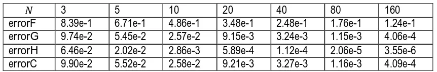
The -norm of error using from ( ) is denoted as errorF, that is,
errorF = ∫ ( ( )− ( )) . (35)
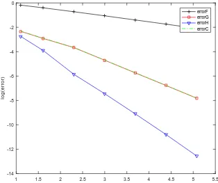
The errors using ( ), ( ) and ( ) are defined similarly and denoted as errorG , errorH and errorC, respectively. The errors at different values of are presented in Table 1 and the graphs using log-log scale are shown in Figure 1.
Table 1: -norm of errors using for different Fourier series
3 5 10 20 40 80 160
Figure 1: The -norm of the errors using partial sums for different Fourier series
As can be seen from Table 1 and Figure 1, the Fourier series of ( ) converges faster than that of ( ), while the Fourier series of ( ) converges faster than that of ( ). ( ) is nearly the same as ( ) because both of them have same degree of smoothness.
Remark 3: The function ( ) can be expanded to a periodic function using polynomial of higher degree following the similar procedures. For example, using polynomial of degree 5 can extend the function to class of , and the corresponding Fourier coefficients is of order and is of order .
References
Baszenski, G., Delvos, F.J., and Tasche, M. (1995). A United Approach to Accelerating Trigonometric Expansions, Computers & Mathematics with Applications, 30, 33-49.
Das, A. (2012). Signal Conditioning, Signals and Communication Technology, Springer, Berlin.
Jones, W.B. and Hardy, G. (1970). Accelerating Convergence of Trigonometric Approximations, Mathematics of Computation, 24, 547-560.
Kido, K. (2015). Digital Fourier Analysis: Fundamentals, Undergraduate Lecture Notes in Physics, Springer, New York. Li, W. (2016). Alternative Fourier Series Expansions with Accelerated Convergence, Applied Mathematics, 7, 1824-1845. Tolstov, G.P. (1976). Fourier Series (translated from Russian by R.A. Silverman), Dover Publications, New York.
1 1.5 2 2.5 3 3.5 4 4.5 5 5.5
log(N)
-14 -12 -10 -8 -6 -4 -2 0
lo
g
(e
rr
o
r)