1D Model vs 2D Model for Flooding Events

1D model vs 2D model for flooding events

M. Morales-Hernández

1,2*

, I. Echeverribar

1

, P. García-Navarro

1

and P.

Brufau

1

1 _{Fluid Mechanics, Universidad Zaragoza/LIFTEC-CSIC, C/María de Luna, 3, Zaragoza, 50018,}

Spain

2 _{Dept. Soil and Water, Aula Dei Experimental Stn., CSIC, Zaragoza, 50080, Spain}

[email protected], [email protected], [email protected], [email protected]

Abstract

One dimensional (1D) shallow water models are widely used for prediction purposes to assess and help river basin administrations and public authorities in the decision-making process. However, their results can be inaccurate since the hypotheses underlying the 1D model are not satisfied during flooding events. On the other hand, two-dimensional (2D) models offer more information to follow the inundation process and the flow properties over floodplains. Despite the well- known higher computational cost of 2D models, they have gained popularity since they can be implemented under GPU cards that allow faster computations, providing more information than 1D models. In this work, two flooding events in the Ebro River (Spain) are analyzed to evaluate the performance of both 1D and 2D shallow water models.

1

Introduction

Prediction tools need to establish a faithful mathematical representation of reality. In case of river flooding, the shallow water system of equations is commonly accepted. In particular, 1D and 2D models are extensively used for this purpose. When dealing with 1D model, the information is averaged along the cross section, hence the wetted area and the discharge in the direction of the flow are solved. The computation is easy and fast, nevertheless when a flooding event occurs, the flow has a two dimensional character since the floodplains and adjacent zones are covered by water and the results may be inaccurate (Echeverribar et al., Journal of Environmental Informatics, 2018, Echeverribar et al., Proceedings of River Flow 2018, 2018). On the other hand, the 2D shallow water model solves the water depth and velocities in both x and y direction of space. The drawback is that, in order to have a correct representation of the topography, a large amount of cells is usually required

Volume 3, 2018, Pages 1449–1456

turning into unaffordable computations. However, in the last years the HPC computing, and in particular, the GPU technology (Lacasta et al., Advances in engineering software, 2014) has reduced this problem.

In this work, we try to answer the question of the convenience of using either the 1D model or the 2D model when dealing with a flooding event. Two real events in the Ebro River (Spain) are considered where some field measurements are provided. Not only the accuracy but also the computational time is analyzed.

2

Domain description and test cases

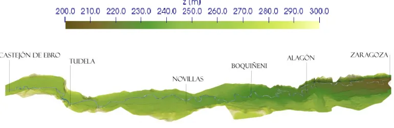
A river reach, 125 km long and 744 km2 in extension, in the middle part of the Ebro River (Spain), between the towns of Castejón de Ebro and Zaragoza is considered in this work (see Figure 1). Both towns have gauging stations that provide the inlet and outlet boundary conditions of our domain.

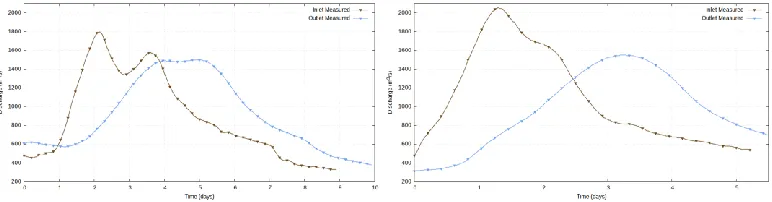
A DTM (5m x 5m) that contains the topographic information as well as different cross sections along the river have been used to generate both computational meshes (for the 1D and 2D model). Moreover, land use maps allow characterizing the roughness (Echeverribar et al., Journal of Environmental Informatics, 2018). Two events are proposed in this work to compare the 1D and the 2D approaches. The first ten day flooding event occurred on June 2008. The discharge hydrograph curve at the inlet station contains two clear peak discharges that are smoothed into a flat ‘plateau’ at the outlet location as the gauging measurements indicate (see Figure 2, left). The inlet hydrograph of the second event has a sharp peak of 2000 m3/s that is laminated into a smooth hydrograph. It took place on January 2010 during almost 6 days (Figure 2, right).

3

1D and 2D models

3.1

1D shallow water equations

The 1D shallow water equations can be expressed in conservative form as follows:

( , )

( , )

( , )

x t

d

x

x

t

dx



_

_



U

F

U

H

U

(1)





2

2 0

1

0

,

,

f

Q

A

Q

g I

A S

S

Q

gI

A





_

_

 

_

_







_{ }



_

_



_

_











 





_

_

_

_





U

F

H

(2)

where

Q

is the discharge,

A

is the wetted cross section area,

g

is the acceleration due to gravity,

0

S

is the bed slope, expressed according to the bed level

z

_b

0

b

z

S

x



 



(3)

and

S

_f represents the friction stress modelled by the Gauckler–Manning law:

2 2

2 4/3

f

Q n

S

A R



(4)

being

R

the hydraulic radius and

n

the roughness coefficient. Accordingly, the water depth is defined as

h

 

z

_s

z

_b being

z

_s the water surface level.

I

₁ and

I

₂ account for hydrostatic pressure forces:

( , ) ( , )

( , )

h x t h x t

 

x

   



















where

  



( , )

x

is the width. It is feasible to write the system (1) into non-conservative form as described in (Morales-Hernández et al., Computers & fluids, 2013), achieving the so-called non-conservative source terms

( , )

( , )

x

( , )

x

x

|

_const

x













U

F

U

H

U

H

U

(6)

3.2

2D shallow water equations

The 2D system of partial differential equations that describe the shallow water equation is:

( )

( )

( )

t

x

y



_



_



_







U

F U

G U

H U

(7)









2 2 2 2 0 0

1

,

,

,

,

2

1

,

,

0,

(

),

(

)

2

T

T _{x y}

x

x y x

T

T

x y y

y x fx y fy

q q

q

h q q

q

gh

h

h

q q

q

q

gh

gh S

S

gh S

S

h

h









_



_











_

_



_

_











U

F

G

H

(8)

where

h

is the water depth defined as before,

q

_x and

q

_y are the unit discharges in x and y directions

respectively and

g

is the gravity acceleration. The bed slope is expressed as follows:

S

_0x

z

S

_0y

z

x

y





 

 





(9)

being

z

the bed level. On the other hand, friction losses are characterized according to Gauckler– Manning’s law:

2 2 2 2

4/3 4/3

fx fy

n u

n v

S

S

h

h





(10)

3.3

Numerical schemes









1 1

1/ 2 1/ 2

n

m m

n n D

i i _{i i}

m m

t

x

 

 

  

 











_



_

 







U

U

e

e

(11)

where



and

e

are the linearized eigenvalues and eigenvectors respectively of the flux Jacobian matrix and

m



2

. It is worth remarking the upwind discretization, denoted by

1/ 2 1/ 2

1

(

|

|)

2

m m i i





 







 . The time step size



t

1D is restricted by the CFL condition:

₁

CFL min

_,

CFL 1

|

|

D m k m

k

x

t











(12)

being



x

de cell size. Analogously, the 2D numerical upwind explicit scheme is written as follows:

1 2 1

(

)

E N n

n n D m

i i k k

k m

i

t

l

S

 

 





_

_







_

_

U

U

e

(13)

The meaning is simple: each cell

i

of size

S

_i will be updated in time according to the arriving

contributions (due to the fluxes and source terms) from the neighbouring edges of length

l

_k. In the

2D framework,

m



3

and

N

_E is the number of adjacent edges for each cell (

N

_E



3

for triangles). Again, the CFL condition limits the time step size. For triangular unstructured meshes, this restriction can be expressed as follows:

_{2 ,}

1,

min(

,

)

CFL min

CFL 1

max

|

|

E

i j i

D m k m i

p N p

k

S

t

l

 





_









_

_









(14)

where



_i is a characteristic distance defined for each cell

i

. More details can be found in (Morales-Hernández et al., Applied Mathematical Modelling, 2016). Additionally, the 2D model is implemented using CUDA to be able to run under GPU cards (Lacasta et al., Advances in engineering software, 2014). This paradigm allows fast computations since a massive parallelization using a large number of cores is used. A particular adaptation for triangular grids is considered in this work, following (Lacasta et al., Advances in engineering software, 2014).

4

Results

The results obtained for the 1D and 2D models are plotted as follows: for each flooding event, the results in terms of discharge evolution at Tudela (close to the inlet location) and Zaragoza (the outlet location) are first plotted in comparison with the corresponding measured hydrograph. Moreover, the evolution in time of water surface level is also evaluated at certain intermediate towns (Tudela, Novillas and Alagón) where some measurements are also provided. Additionally, the computational time required by each model is displayed.

4.1

Case 1

4.2

Case 2

Figure 3: Case 1: measured and simulated hydrographs at Tudela (left) and Zaragoza (right)

Figure 4: Case 1: measured and simulated water surface level at Tudela (left), Novillas (middle) and Alagón (right)

4.3

Computational time

Table 1 shows the computational time required by each model. As expected, the 1D model is much faster than the 2D model. However, note that the latter is able to provide very accurate results in less than real time. In particular, in the domain of study of this work, one day of a flooding event is computed in less than one hour when using the 2D model.

Model Computational time (s)

Case 1 Case 2

1D 73,16 45,22

2D 21178 13896

Table 1: Computational time achieved by each model

5

Conclusions

A comparison between 1D and 2D models for two real flooding events in the Ebro River (Spain) has been carried out. In terms of accuracy, the 2D model achieves very good results with respect to the measured level surface. Moreover, the output hydrograph is precisely estimated as well. However, the 1D model overestimates the water level at all the intermediate locations, providing results with 3m of difference with respect to the measured level. Additionally, the time of arrival of the peak discharges and their magnitude is not well captured. Regarding the computational time, the 1D model is certainly faster than the 2D approach. However, it is worth mentioning that the 2D model is able to simulate 1 day in less than 1 hour, making it a potential tool to be incorporated for prediction purposes, demonstrating an attractive compromise between accuracy and computational time. The use of coupled 1D-2D models is still under research in order to have a complete comparison of river flooding prediction numerical simulation.

6

Work in progress

We are trying to adapt the 1D model in order to consider other modifications that allow us to compute in a better way the behaviour of the flooding evolution, not only in terms on peak discharges and the magnitude of water surface level but also in the time of arrival.

References

Echeverribar, I., Morales-Hernández, M., Brufau, P. and García-Navarro, P. (2018). Numerical simulation of 2D real large scale floods on GPU: the Ebro River. Proceedings of River Flow 2018, 9th international conference on fluvial hydraulics. Lyon-Villeurbanne, France

Echeverribar, I., Morales-Hernández, M., Brufau, P. and García-Navarro, P. (2018) Generation and calibration of an optimal computational mesh for the flood inundation prediction in the Ebro River (Spain). Submitted to Journal of Environmental Informatics.

Morales-Hernández, M., Petaccia, G., Brufau, P. and García-Navarro, P. (2016). Conservative 1D–2D coupled numerical strategies applied to river flooding: The Tiber (Rome), Applied Mathematical Modelling, 40:3 (2016) 2087-2105.

Lacasta, A., Morales-Hernández, M., Murillo, J., and García-Navarro, P. (2014). An optimized GPU implementation of a 2D free surface simulation model on unstructured meshes, Advances in engineering software 78, 1-15.

Murillo, J. and García-Navarro, P. (2010). Weak solutions for partial differential equations with source terms: Application to the shallow water equations. Journal of Computational Physics, 229:11 4327–4368.