ISSN: 2008-6822 (electronic)
http://dx.doi.org/10.22075/ijnaa.2016.458
Differential transform method for a nonlinear system
of differential equations arising in HIV infection of
CD
4
+
T
cells
Javad Damirchi∗, Taher Rahimi Shamami
Department of Mathematics, Faculty of Mathematics, Statistics and Computer Science, Semnan University, Semnan, Iran (Communicated by A. Ebadian)
Abstract
In this paper, differential transform method (DTM) is described and is applied to solve systems of nonlinear ordinary differential equations which is arising in HIV infections of cell. Intervals of validity of the solution will be extended by using Pade approximation. The results also will be compared with those results obtained by Runge-Kutta method. The technique is described and is illustrated with one numerical example. The numerical results shown that the reliability and efficiency of the method.
Keywords: Differential transform method; Systems of nonlinear ordinary differential equations; Pade approximation; Fourth order Runge-Kutta method.
2010 MSC: Primary 47H10; Secondary 47H09.
1. Introduction
Many mathematical models have proposed Vivo dynamical of T cell and HIV (Human Immunodefi-ciency Virus) interaction. Our interesting model is the one that is presented in [1], which is explained by the following nonlinear system of ordinary differential equations:
dT
dt =p−αT +rT(1− T+I
Tmax)−kV T,
dI
dt =kV T −βI, dV
dt =N βI−γV.
(1.1)
∗Corresponding author
Email addresses: [email protected](Javad Damirchi),[email protected](Taher Rahimi Shamami)
with the following initial conditions,
T(0) =r1, I(0) = r2, V(0) =r3,
where T(t), I(t) and V(t) denoted the concentration of susceptible CD4+T cells, infected CD4+T
cells by the HIV viruses, and free HIV virus particles in the blood, respectively. Parametersα,β, and γ are natural turn-over rates of uninfected T cells, infected T cells, and virus particles, respectively. The logistic growth of the healthyCD4+T cells is now described by rT(1− T+I
Tmax) , and proliferation
of infected CD4+T cells is neglected. The term kV T describes the incidence of HIV infection of
healthy CD4+T cells, where k > 0 is the infection rate. Each infected CD4+T cell is assumed to produceN virus particles during its lifetime, including any of its daughter cells. The body is believed to produceCD4+T cells from precursors in the bone marrow and thymus at a constant rate . When
stimulated by antigen or mitogen, cells multiply through mitosis with a ratep. Tmax is the maximum level of cell concentration in the body [2, 5]. In this paper, a new kind of analytical approach for a non-linear system of ordinary differential equations called Differential transformation method (DTM) is addressed and used to approximate solutions for a well-known non-linear system. The differential transformation method is a kind of analytical technique based on the Taylor series expansion. This method constructs an analytic approximation to the solution, polynomial form. The concept of differential transform method was first proposed by Zhou and was applied to solve linear and nonlinear initial value problems in electric circuit analysis [6]. Chen and Liu applied this method to solve two-boundary-value problems [7]. Jang, Chen and Liu used two-dimensional differential transform method to solve partial differential equations [8]. Yu and Chen applied the differential transformation method for optimization of the rectangular fins with variable thermal parameters [9, 10]. Unlike the traditional high order Taylor series method that requires many symbolic computations, the differential transform method is an iterative procedure for obtaining Taylor series solutions. This method will not consume too much computer time when applying to non-linear or parameter varying systems.
2. Basic Idea of Differential Transform Method
As in Refs. [7, 8, 11, 12, 13], the differential transformation is based on some elementary definitions, and some statements, which will be stated as follows.
Definition 2.1. The one-dimensional differential transform of a function c(x) is defined as:
C(k) = 1 k![
∂k
∂xkc(x)]x=x0,
where c(x) is analytic and continuously differentiable with respect to x on the domain of interest and C(k) is the transformed function, which is called T-function.
Definition 2.2. The inverse differential transform of C(k) is defined as follows:
c(x) = ∞
X
k=0
C(k)(x−x0)k,
when x0 = 0, Definitions 2.1 and 2.2 turn to the followings:
C(k) = 1 k![
∂k
c(x) = ∞
X
k=0
C(k)xk, (2.2)
where c(x) is the original function and C(k) is the T-function. Substituting (2.1) into (2.2) leads to
c(x) = ∞
X
k=0
1 k![
∂k
∂xkc(x)]x=0x k.
In real applications, finite form of the series (2.2) will be considered as follows:
c(x) = n X
k=0
C(k)xk.
From Definitions 2.1 and 2.2, it is readily proved that the transformed functions comply with the basic mathematical operations [9, 10, 13]. These statements are illustrated in the Table 1.
TABLE 1
Transformation of some functions [9] Original function Transformed function
c(t)=u(t)±v(t) C(k)=U(k)±V(k) c(t)=au(t) C(k)=aU(k) c(t)=∂t∂u(t) C(k)=(k+1)U(k+1)
c(t)=u(t)v(t) C(k)=Pk
r=0U(r)V(k-r)
c(t)=elt C(k)=lk k!
c(t)=sin(wt+a) C(k)=wkk! sin(kπ2 +a) c(t)=cos(wt+a) C(k)=wkk! cos(kπ2 +a)
3. Pade approximation
Here we will investigate the construction of the Pade approximants for the functions studied. Pade approximation of a function is given by the ratio of two polynomials. The coefficients of the polyno-mial in the numerator and denominator are determined by using the coefficients in the Taylor series expansion of the function. Suppose that we are given a power seriesP∞
i=0cit
i representing a function so thatf(x) =P∞
i=0citi.
The Pade approximation of a function is a rational fraction and a notation for such a Pade approximation is shown as:
[m, n] = Pm(x) Qn(x)
= a0+a1t+a2t
2+...+a
mtm b0+b1t+b2t2 +· · ·+bntn
=c0+c1t+c2t2+· · ·+cm+ntm+n, (3.1)
where Pm(x) and Qn(x) are polynomials of degree at most m and n. We impose the normalization condition Qn(0) = b0 = 1, therefore, there are m+ 1 independent numerator coefficients and n
independent denominator coefficients, making m+n+ 1 unknown coefficients in all. This number suggests that normally the ought to fit the power series in equation (3.1) through the orders and finally we know that the Pade approximation is uniquely determined.
The construction of [m, n] approximation involves only algebraic operations. Each choice of m degree of the numerator and n degree of the denominator, leads to an approximation. The major difficulty in applying this technique is how to direct the choice in order to obtain the best approximation. This requires a criterion which dictates the choice of approximation, depending on the shape of the solution. A criterion which has worked well here is the choice of [m,n] approximation such that m=n . Using the symbolic computation software MATHEMATICA, we directly employ the command ”Pad Approximation” about the point x =x0 to generate the Pad approximation of
4. Applications
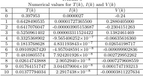
Considering the following values, the differential transformation of the system (1.1) can be con-structed as follows:
TABLE 2
Numerical values for variables of system (1.1)
Variable Numerical Value Variable Numerical Value Variable Numerical Value
T(0) 0.1 α 0.02 k 0.0027
I(0) 0 β 0.3 Tmax 1500
V(0) 0.1 r 3 N 10
p 0.1 γ 2.4
T(k+ 1) = k+11 (0.1−0.02T(k) + 3T(k)− 1 500
Pk
j=0T(j)T(k−j)
− 1 500
Pk
j=0T(j)I(k−j)−0.0027
Pk
j=0V(j)T(k−j)),
I(k+ 1) = k+11 (0.0027Pk
j=0V(j)T(k−j)−0.3I(k)),
V(k+ 1) = k+11 (3I(k)−2.4V(k)).
Substituting the numerical values of T(0),I(0) and V(0) from Table 2, into (3.1), results in the following values:
TABLE 3
Numerical values forT(k),I(k) andV(k) k T(k) I(k) V(k) 0 0.397953 0.0000027 -0.24 1 0.6428490535 0.00001727365500 0.2880405000 2 0.6417076047 -0.000003905153687 -0.2304151263 3 0.5250961402 0.000003311524422 0.1382461469 4 0.3325368902 -9.565406252×10⁻⁷ -0.06635616360
5 0.1813768628 4.831193843×10⁻⁷ 0.02654198717
6 0.09109267420 -4.957048591×10⁻⁸ -0.009099902836
7 0.4810805574 7.924201926×10⁻⁸ 0.002729952262 8 0.02614743888 2.9052940×10⁻⁸ -0.0007279608559
9 0.01764151747 3.044379004×10⁻⁸ 0.0001747193213
10 0.01377794034 2.2917438×10⁻⁸ -0.00003811227634
Therefore, the solution of the system (1.1) is given by:
T(t) = 0.1 + 0.397953t+ 0.6428490535t2+ 0.6417076047t3+ 0.5250961402t4+ 0.3325368902t5 + 0.1813768628t6+ 0.09109267420t7+ 0.4810805574t8+ 0.02614743888t9
+ 0.01764151747t10+ 0.01377794034t11+...,
I(t) = 0 + 0.0000027t+ 0.00001727365500t2−0.000003905153687t3+ 0.000003311524422t4 −9.565406252×10⁻⁷t5+ 4.831193843×10⁻⁷t6 −4.957048591×10⁻⁸t7
+ 7.924201926×10⁻⁸t8+ 2.9052940×10⁻⁸t9+ 3.044379004×10⁻⁸t10+ 2.2917438×10⁻⁸t11+...,
In the above results, six terms approximations are considered, because the rest of the terms are too small therefore,
T(t) = 0.1 + 0.397953t+ 0.6428490535t2+ 0.6417076047t3+ 0.5250961402t4+ 0.3325368902t5 + 0.1813768628t6+,
I(t) = 0 + 0.0000027t+ 0.00001727365500t2−0.000003905153687t3+ 0.000003311524422t4 −9.565406252×10⁻⁷t5+ 4.831193843×10⁻⁷t6,
V(t) = 0.1−0.24t+ 0.2880405000t2−0.2304151263t3+ 0.1382461469t4−0.06635616360t5 + 0.02654198717t6.
Now, the Pade approximation [4,4] are calculated as follows:
Tpade(t) =
0.1−1.224115531t−3.460113984t2−1.802983875t3−0.490931507t4 1−16.22068531t+ 23.52107342t2−14.07521016t3+ 3.603023454t4 ,
Ipade(t) =
0.000027t+ 0.000005102627t2−0.0000242556t3−0.00000336726t4
1−0.4507788263t+ 0.4653299318t2−0.01485902265t3+ 0.3291816479t4,
Vpade(t) =
0.1−0.120287067t−0.06212670482t2−0.0166266799t3−0.002041025824t4
1−1.197129325t+ 0.6139724293t2 −0.163201268t3+ 0.01950991258t4 ,
5. Fourth Order Runge-Kutta Method
The system (1.1) in the vector form can be written as follows,
{Y}= dY
dt =F(t, Y), t ≥0, with initial condition
Y(0) =Y0,
where
Y =
T I V
,
F(t, Y) =
f1(t, T, I, V)
f2(t, T, I, V)
f3(t, T, I, V)
=
p−αT +rT(1− T+I
Tmax)−kV T,
kV T −βI N βI−γV
,
Y0 =
T(0) I(0) V(0)
By using Fourth order Runge-kutta method for the system (1.1) we have
Yi+1 =Yi+ 1
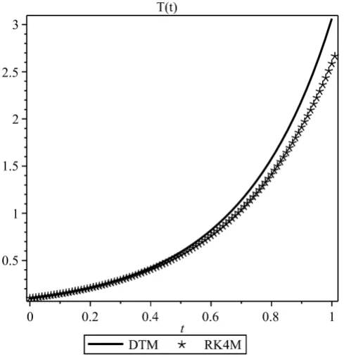
Figure 1: Numerical comparison for determination ofT(t) between DTM and Runge-Kutta method
where
K1 =
k11 k21 k31
, K2 =
k12 k22 k32
, K3 =
k13 k23 k33
, K4 =
k14 k24 k34 ,
kj1 =h(ti+Ti+Ii+Vi), j = 1,2,3,
kj2 =hfj(ti+ h 2, Ti+
k11
2 , Ii + k21
2 , Vi+ k31
2 ), j = 1,2,3, kj3 =hfj(ti+
h 2, Ti+
k12
2 , Ii + k22
2 , Vi+ k32
2 ), j = 1,2,3, kj4 =hfj(ti+h, Ti+k13, Ii+k23, Vi+k33), j = 1,2,3,
where his the step size.
The above equations can be expressed an explicit form as the following:
Ti+1
Ii+1
Vi+1
= Ti Ii Vi + 1 6{ k11 k21 k31
+ 2 k12 k22 k32
+ 2 k13 k23 k33 + k14 k24 k34
}, i= 0,1,2, ...
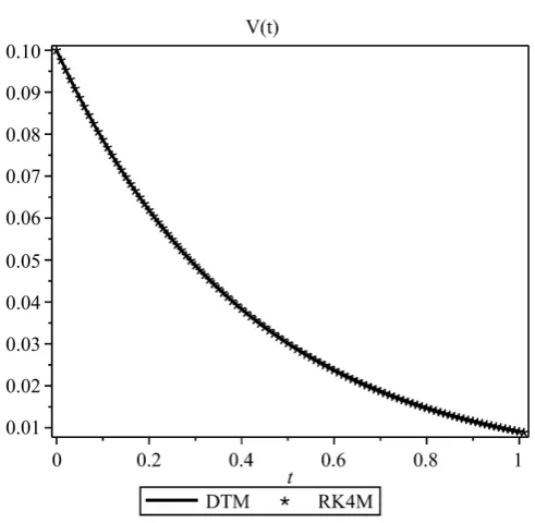
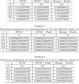
Consideringh= 0.01 the solutions of the Runge-kutta method are in good agreement with those of DTM. The numerical results are shown in Tables 4, 5 and 6. In addition, the solutions of DTM and Runge-kutta method are plotted in Figure 1, 2, 3.
TABLE 4
Figure 2: Numerical comparison for determination ofI(t) between DTM and Runge-Kutta method
t DT M DT M−P ade Runge−Kutta
0 0.1 0.1 0.1
0.2 0.2116376961 0.2116378080 0.2088080121 0.4 0.4228059053 0.4228270719 0.4062401504 0.6 0.8214427381 0.8220867977 0.7644222857 0.8 1.580090941 1.589428602 1.414040889 1 3.068328771 3.167027048 2.591573918
TABLE 5
Numerical comparison for determination ofI(t) for different values oft
t DT M DT M−P ade Runge−Kutta
0 0 0 0
0.2 0.000006064727822 0.000006064727837 0.00000603270115 0.4 0.00001339079678 0.00001339080558 0.00001315833510 0.6 0.00002195290254 0.00002195342310 0.00002122376663 0.8 0.00003183956342 0.00003185446433 0.00003017737081 1 0.00004335422355 0.00004394009567 0.0000400376991
TABLE 6
Numerical comparison for determination ofV(t) for different values oft
t DT M DT M−P ade Runge−Kutta
0 0.1 0.1 0.1
0.2 0.06187984770 0.06187984749 0.06187984331 0.4 0.03829494797 0.03829494731 0.03829488788 0.6 0.02370481149 0.02370483059 0.02370455013 0.8 0.01468108240 0.01468128654 0.01468036373 1 0.009102264150 0.009103435566 0.009100845022
6. Conlcusion
In this paper, the HIV Infection of CD4+T cells model is solved by DTM and fourth order Runge-Kutta methods, successfully. The results obtained by these two methods are plotted in Figure 1. Comparison of these two methods can be resulted from Tables 4, 5, 6, or figure 1. Results of these two methods are close at the beginning of the intervals, and the solutions get to lose the common figures. The fourth part of Figure 1 and Tables 4,5,6 show that as the time passes, the concentration of number of healthy cells which is denoted byT(t) and the HIV viruses which are denoted by I(t) is the worth and the numbers of free HIV viruses which are denoted by V(t) have more digits in common. Behavior of T(t) and I(t) are almost the same, and it increases as the time increases, but the rate of increasing of I(t) is less than those ofT(t) and V(t) decrease as the time increases. Computations are performed by using Maple 13 package.
References
[1] A.S. Perelson, D.E. Kirschner and R.D. Boer,Dynamics of HIV infection CD4+T cells, Math. Biosci. 114 (1993) 81–125.
[2] A.S. Perelson and P.W. Nelson, Mathematical analysis of HIV-I Dynamics in Vivo, SIAM Rev. 41 (1999) 3–44. [3] L. Wang and M.Y. Li, Mathematical analysis of the global dynamics of a model for HIV infection of CD4+T
cells, Math. Biosci. 200 (2006) 44–57.
[4] B. Asquith and C.R.M. Bangham,The dynamics of T-cell fratricide: application of a robust approach to mathe-matical modelling in immunology, J. Theoret. Bio. 222 (2003) 53–69.
[5] M. Nowak and R. May,Mathematical biology of HIV infections: antigenic variation and diversity threshold, Math. Biosci. 106 (1991) 1–21.
[6] X. Zhou, Differential Transformation and its Applications for Electrical Circuits, Huazhong University Press, Wuhan, China, (1986) (in Chinese).
[7] C.L. Chen and Y.C. Liu, Differential transformation technique for steady nonlinear heat conduction problems, Appl. Math. Comput. 95 (1998) 155–164.
[9] L.T. Yu and C.K. Chen, The solution of the Blasius equation by the differential transformation method, Math. Comput. Model. 28 (1998) 101–111.
[10] L.T. Yu and C.K. Chen,Application of taylor transformation to optimize rectangular fins with variable thermal parameters, Appl. Math. Model. 22 (1998) 11–21.
[11] F. Ayas,On the two-dimensional differential transform method, Appl. Math. Comput. 143 (2003) 361–374. [12] F. Ayas,Solutions of the system of differential equations by differential transform method, Appl. Math. Comput.
147 (2004) 547–567.