Control Strategies for Shunt Active Power Filter for Three-Phase Four-Wire System

(1)

24

Available online at www.ijiere.com

International Journal of Innovative and Emerging

Research in Engineering

e-ISSN: 2394 – 3343 p-ISSN: 2394 – 5494

Control Strategies for Shunt Active Power Filter for

Three-Phase Four-Wire System

1

_{Jaykumar Prakashchandra Topiwala,}

2

_{Prof. Bijal K. Mehta}

Department of electrical engineering, Sarvajanik College of Engineering and Technology, Surat, Gujarat, India-395001

ABSTRACT:

Most of the pollution issues created in power systems are due to the non-linear characteristics and fast switching of power electronic equipment. So that shunt active power filter is used to eliminate load current harmonics and reactive power compensation. Strategies for extracting the three-phase reference currents for shunt active power filters are compared. Here the performance of compensating current extraction algorithms will be simulated using Matlab/Simulink. Almost four compensating strategies such as instantaneous active reactive power theory, modified p-q, unity power factor (UPF) method, perfect harmonic cancellation (PHC) are used.

Keywords:p-q theory, modified p-q , UPF ,PHC, transient analysis

I. INTRODUCTION

Power quality is very broad in nature. It covers all subject of power system engineering from transmission and distribution to end-user problem. There are many reasons for bad power quality. There are various solutions for power quality improvement. One solution is to use line-conditioning systems that counteract the power system disturbances. It includes passive filter, active filter and hybrid filters. The active power filters (APF) is an important and flexible alternative to compensate for current and voltage disturbances. Depending on the power-circuit configuration and connections APF can be divided into three types shunt, series and hybrid APF. Shunt APF compensate load current harmonics by injecting equal and opposite phase harmonic current and operates as a current source [1]. Shunt APF are used to compensate load current related issues, such as load reactive power, current harmonic, current unbalances and neutral current[2]. As shown in Fig. 1, shunt APF consists of three main parts as PWM converter (power processing), PWM controller, Active filter controller (signal processing).

Figure 1. Shunt APF configuration [3]

In many cases, the neutral currents are potentially damaging to the neutral conductor and the transformer to which it is connected. Three phase four wire APF have been proposed by researchers as a solution to these problems [3]. The four legs VSI have more degree of freedom to eliminate the neutral current as well as require small capacitor of less capacitance. Active filter controller (signal processing) includes various control strategies to generate reference current for VSI to compensate the distortion in source current.

II. REFERENCESIGNALGENERATION

Development of reference signals in terms of currents is the most important part of the shunt APF controller and it affects their rating, transient and steady-state performance. The control strategies used are based on

1. Frequency-domain control techniques and 2. Time-domain control techniques

(2)

25 time domain are depends on instantaneous derivation of compensating commands in the form of current signals from distorted and harmonic-polluted current signals. There are very large numbers of control techniques in the time domain. Almost four compensating strategies which are widely used are instantaneous reactive power method (p-q method), Modified p-q or cross-product method, Unity power factor (UPF) method, Perfect harmonic cancellation (PHC) method. In all method voltage at the point of common coupling (PCC, which is usually secondary of distribution transformer) and load current are sensed. These signals are given to the different control strategies to obtain reference compensating signals. These compensating signals are given to PWM controllers.

 Instantaneous reactive power method (p-q method)

The instantaneous reactive power (p-q) theory has been widely used and is based on "α-β-0" transformation of instantaneous measured voltage vas, vbs, vcs and load current signals ia, ib, ic to extract compensating signals.

Figure 2. Block diagram of three phase p-q theory[2][4]

 Modified p-q or cross-product method

The instantaneous reactive power given by the modified theory is different from that defined by the original theory including a zero-sequence voltage and current. The difference in their “mapping matrices”[5]. The difference and features of the two theories are summarized as follows:

1. The original theory considers the zero-sequence circuit as a “independently” from the α phase circuit and the β phase circuit, and therefore it would be suitable for applications on the α-β-0 systems.

2. The modified theory deals with the zero-sequence circuit, the α phase circuit and the β phase circuit “equally,” and therefore it would be suitable for applications on the a-b-c coordinate as well [2].

Figure 3 Block diagram of modified p-q theory [5]

[

x0

xα xβ

]

=

√

2

3∗

[

1 √2 1 √2 1 √2

1 −1

2 −

1 2

0 √3

2 − √3 2

]

∗

[

xa xb

xc

]

[

p0 pα β qα β

]

=

[

v0 0 0

0 vα vβ

0 vβ −vα

]

[

i0 iα iβ

]

Clarkes Transformation _{Instantaneous power} calculation

[

ic0

icα

icβ

]

= 1

vα

2 +vβ

2

[

vα

2 +vβ

2

0 0

0 vα vβ

0 vβ −vα

]

[

−i0 − ̃p+p̄loss

−qα β

]

[

ica icb icc

]

=

√

2

3

[

1 √2 1 0 1 √2 −1 2 √3 2 1

√2 − 1

2 −

√3 2

]

[

ic0 icα icβ

]

ic0=− (ica+icb+icc)

Ica Icb Icc Ico Low Pass Filter PI cont. -1 Vref +

-Vdc ̄ ploss + -+ ̄p

Inverse Clarkes Transformation p=p

0+pαβ

α β current calculation

q αβ

-q_αβ

− ̃p+p̄loss

v_αβ0 i_αβ0

vabcs

iabc

[

x0 xα xβ

]

=

√

2

3∗

[

1 √2 1 √2 1 √2

1 −1

2 −

1 2

0 √3

2 − √3 2

]

∗

[

xa xb

xc

]

[

p q0

qα

qβ

]

=

[

v0 vα vβ

0 −vβ vα

vβ 0 −v0

−vα v0 0

]

[

i0

iα

iβ

]

Clarkes Transformation Instantaneous power calculation

[

ic0

icα

icβ

]

= 1

v0 2

+vα

2 +vβ

2

[

v0 0 vβ −vα

vα −vβ 0 v0

v_β v_α −v0 0

]

[

− ̃p+p̄loss

q0

qα

qβ

]

[

ica icb icc

]

=

√

2

3

[

1

√2

1 0

1

√2 − 1 2

√3 2

1

√2 − 1

2 −

√3

2

]

[

ic0 icα i_cβ

]

ic0=− (ica+icb+icc)

Low Pass Filter PI

cont. Vref +

-Vdc ̄ ploss - + -̄p

Inverse Clarkes Transformation p=p

0+pαβ

q_αβ0

q αβ0

− ̃p+p̄loss

(3)

26

 Unity power factor(UPF) method

The compensating strategy known as the unity power factor (UPF) method has the objective that the load and the compensator as a resistance for source. This method is sometimes called as the “voltage synchronization method” because the reference source current has zero degree phase shift with the PCC voltage space vector [6]

Figure 4 Block diagram of unity power factor theory [6]

 Perfect harmonic cancellation(PHC) method

It is used to compensate all the harmonic currents components, fundamental reactive power of the load and imbalance. The voltage at PCC will be given to the PLL to get the fundamental positive sequence voltage signals.

Figure 5 Block diagram of perfect harmonic cancellation theory [5] III.SIMULATION

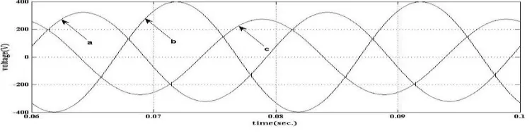
Here we have considered three single phase non-linear loads connected to RL load. The simulation parameter are source voltage Vs=400V; 50Hz, Source impedance Rs=0.02Ω; Ls=50μH, DC link capacitor Cdc=1000μF; Vdc=900V, Coupling reactor Lf=1mH.

A. Shunt APF Under Different Source And Load Condition

Case-1: Ideal supply and balanced non-linear load. In this case supply voltage is ideal one. The value of load impedance Rl=25Ω; Ll=100mH are in series.

[

x0 xα xβ

]

=

√

2

3∗

[

1 √2 1 √2 1 √2

1 −1

2 −

1

2

0 √3

2 − √3 2

]

∗

[

xa xb

xc

]

v_αβ0

i_αβ0

[

p0

pα β

]

=

[

v0 0 0 0 vα vβ

]

[

i₀

iα iβ

]

[

is0

i_sα

i_sβ

]

= ̄p+p̄loss (v0

2

+vα

2

+vβ

2

)_dc

[

v₀ vα

vβ

]

[

isa isb

isc

]

=

√

2

3

[

1

√2

1 0

1

√2 − 1

2

√3 2

1

√2 − 1

2 −

√3 2

]

[

is0 isα

isβ

]

is0=− (isa+isb+isc)

Mean PI

cont. Vref +

-Vdc

̄

ploss+ + ̄p Inverse Clarkes Transformation

p=p₀+p_αβ

̄p+p̄loss

vα β0

iabcs -+

iabcn

iabcns iCabcn

iabc

vabcs

u

2

Mean

[

x0 xα xβ

]

=

√

2

3∗

[

1 √2 1 √2 1 √2

1 −1

2 −

1 2

0 √3

2 − √3 2

]

∗

[

xa xb xc

]

v

αβ0

i

αβ0

[

p0

pα β

]

=

[

v0 0 0 0 vα vβ

]

[

i0 iα iβ

]

[

is0

i_s_α i_s_β

]

= ̄ p+p̄_loss v_α2₁+v_β2₁

[

0

v_α₁ vβ1

]

[

isa isb isc

]

=

√

2

3

[

1

√2 1 0 1

√2 − 1 2

√3 2 1

√2 − 1

2 −

√3 2

]

[

is0 isα isβ

]

is0=− (isa+isb+isc)

Low Pass Filter PI

cont. Vref +

-Vdc

̄

ploss ₊ + ̄p

Inverse Clarkes Transformation

p=p₀+p_αβ

α β current calculation PLL

v

_abc1

̄p+p̄loss

vα β1

iabcs -+

iabc0

iabc0s iCabc0

iabc

vabcs

(4)

27 Figure 6 Source voltages for case-1

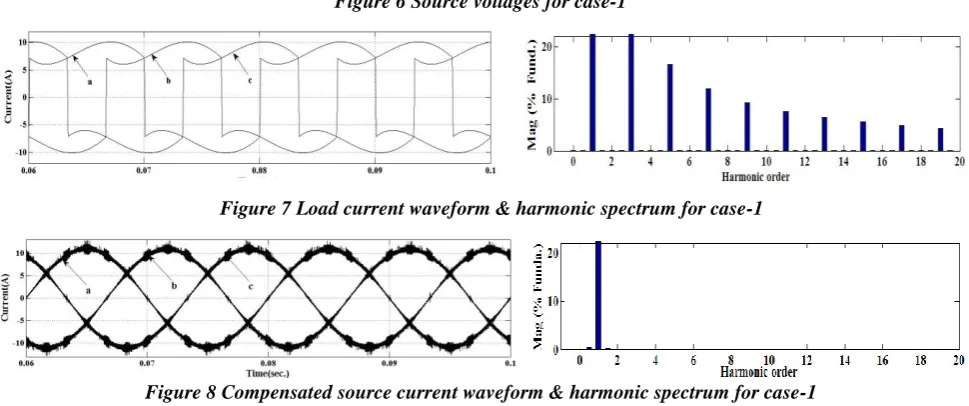
Figure 7 Load current waveform & harmonic spectrum for case-1

Figure 8 Compensated source current waveform & harmonic spectrum for case-1

Under all the control strategies we get the same source current. The result of simulation is in the following table

TABLE 1 SUMMARY OF SIMULATION RESULTS FOR CASE-1

Parameter Without APF For all methods Load Current(A) 7.723 7.723

Source current (A) 7.723 7.687

Active Power (W) 5262 5291

Reactive Power (VAr) 929.6 -29.31

Source Current THD(%) 39.19 3.07

Third Harmonic(%) 27.10 0.03

Hence all control strategies have given similar performance under balanced and sinusoidal source voltage condition and hence all the strategies are equivalent.

Case-2: Balance undistorted supply: unbalanced non-linear load. Here we have considered three single phase unbalanced non-linear load. In which the total unbalance is 25% of negative-sequence to positive-sequence load current. The supply voltages are balanced and undistorted in each phase. The source voltage is same as in case-1 and uncompensated load current is as below

Figure 9 Waveform & harmonic spectrum of load current for case-2

As shown in Fig. 9 load current and source current are same without APF with rms of positive sequence fundamental current is 39.07A and THD is 32.57% is in verse phase B. The source current after compensation is shown in below figures.

 p-q method

Figure 10 Waveform & harmonic spectrum of source current after compensation by p-q method for case-2

By p-q method shunt APF can cancels the current harmonics generated by nonlinear load in case-2. The THD of source current is 3.58% with fundamental value of 27.56A in phase b.

(5)

28 Figure 11 Waveform & harmonic spectrum of source current after compensation by modified p-q method for case-2

By modified p-q method shunt APF can cancels the current harmonics generated by nonlinear load in case-2. The THD of source current is 3.70% with fundamental value of 26.7A in phase b.

 UPF method

Figure 12 Waveform & harmonic spectrum of Source current after compensation by UPF method for case-2 By UPF method shunt APF can cancels the current harmonics generated by nonlinear load in case-2. The THD of source current is 3.27% with fundamental value of 26.68A in phase b.

 PHC method

Figure 13 Waveform & harmonic spectrum of Source current after compensation by PHC method for case-2

By PHC method shunt APF can cancels the current harmonics generated by nonlinear load in case-2. The THD of source current is 1.81% with fundamental value of 26.7A. The result table are as follows

Table 2 Summary of Simulation Results for Case-2

Parameter Without APF p-q

Modified

p-q UPF PHC Ia(A) 30.89 27.56 27.19 27.18 27.19 Ia THD(%) 27 3.58 4.10 2.62 2.12

Ib(A) 39.07 27.56 26.7 26.68 26.7 Ib THD(%) 32.57 3.58 3.70 3.27 1.81 Ic(A) 16.66 27.72 27.35 27.33 26.35 Ic THD(%) 23.37 3.09 3.73 1.72 1.55 Active Power(W)*104 _1.85 _1.901 _1.859 _{1.868 1.864} Reactive Power(VAr) 4373 -24.6 1.233 45.88 -25.35

Third Harmonic (%) 21.58 1.38 1.43 2.89 1.39

Among above mentioned ideal source voltage and unbalanced load all method produces balanced source currents. The increased source active power and source current are because of inverter losses. All method can reduce third harmonic below 4% and hence IEEE519 standard s satisfied.

Case-3: Unbalance undistorted supply: balanced non-linear load

The unbalanced in source voltage is 23.1% of negative sequence to positive-sequence voltage at 1000 _{phase shift. The} source voltage and uncompensated load current are shown below for case-3

Figure 14 Source voltages for case-3

(6)

29 Figure 15 Waveform & harmonic spectrum of Load current for case-3

As shown in Figure 15 load current and source current are same without APF with rms of positive sequence fundamental current is 8.501A and THD is 32.76% is in phase b. The source current after compensation is shown in below figures.

 p-q method

Figure 16 Waveform & harmonic spectrum of Source current after compensation by p-q method for case-3

By p-q method shunt APF cannot cancels the current harmonics generated by nonlinear load in case-3. The THD of source current is 22.65% with fundamental value of 9.65A in phase b.

 Modified p-q method

Figure 17 Waveform & harmonic spectrum of Source current after compensation by modified p-q method for case-3

By modified p-q shunt APF cannot cancels the current harmonics generated by nonlinear load method in case-3. The THD of source current is 22.81% with fundamental value of 9.082A in phase b.

 UPF method

Figure 18 Waveform & harmonic spectrum of Source current after compensation by UPF method for case-3

By UPF method shunt APF cannot cancel the current harmonics generated by nonlinear load in case-3 but unbalanced from the source current cannot be removed. The THD of source current is 2.31% with fundamental value of 8.296A in phase-b.

 PHC method

Figure 19 Source current after compensation by PHC method for case-3

(7)

30

Table 4 Summary of Simulation Results for Case-3

Parameter Without APF p-q

Modified

p-q UPF PHC

Ia(A) 6.45 8.662 8.665 7.129 8.793

Ia THD(%) 23.50 23.46 23.62 2.13 1.91

Ib(A) 8.501 9.65 9.082 8.296 8.958

Ib THD(%) 32.76 22.65 22.81 2.31 1.88

Ic(A) 10.03 8.873 8.87 10.19 8.88

Ic THD(%) 20.08 23.18 23.28 2.25 1.56

Active Power(W) 5264 6138 6116 5808 6153

Reactive Power(VAr) 942.3 65.16 30.42 9.781 -3.571

Third Harmonic (%) 27.09 23.35 22.71 2.89 0.88

Among above mentioned non-ideal source voltage conditions, only PHC produces balanced source currents and reduce third harmonic below 4% and hence IEEE519 standard is satisfied. And in UPF method THD is improved to 2.31% and IEEE519 standard are satisfied. The increased source active power and source current are because of inverter losses.

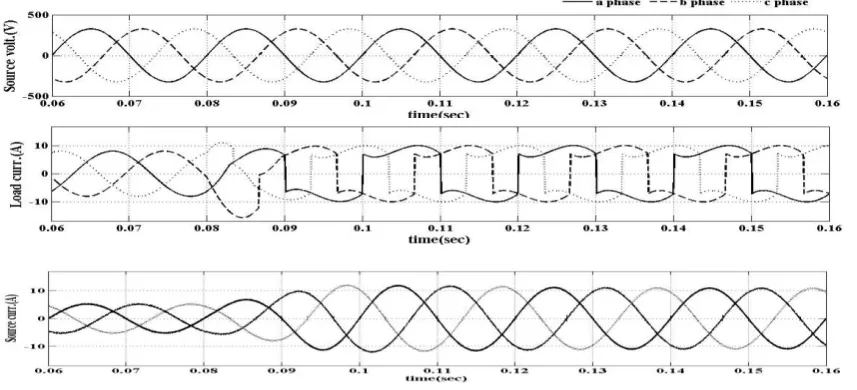
B. Transient Performance of Shunt Active Power Filter

The transient performance of shunt APF is shown below. Initially balanced linear load is connected to the three phase sinusoidal source. The value of linear-load resistance Rl=25Ω and inductance Ll=100mH are connected in series in each phase. At 0.08 sec load is changed from linear-load to non-linear load. Nonlinearity of current can be seen in the load current whereas the source current is observed as sinusoidal because of the shunt APF. Here we have considered three single phase non-linear loads. The value of load resistance Rl=25Ω and inductance Ll=100mH are in series in each phase.

Figure 20 Transient Performance of Shunt Active Power Filter

Transient performance can be observed in capacitor voltage. Settling time is time required for the capacitor to reach and stay within a range of the final value. Here capacitor steady state final voltage is 900V and range chosen is 0.5%. Transient performance under various control strategies are shown as follows.

(8)

31

Figure 21 Variation in capacitor voltage for p-q method

The change in load is taken at .08sec and capacitor will reach at 895V at 0.1159sec. Hence settling time taken by shunt APF in this method is, ∆t = 0.1159 - 0.08 = 0.0359sec.

 Modified p-q method

Figure 22 Variation in capacitor voltage for modified p-q method

 UPF method

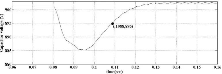
Figure 23 Variation in capacitor voltage for UPF method

 PHC method

Figure 24 Variation in capacitor voltage for PHC method

The change in load is taken at 0 .08sec and capacitor will reach at 895V at 0.1157sec. Hence settling time taken by shunt APF in this method is, ∆t = 0.1157 - 0.08 = 0.0357sec.

From the above results we can say that upf method is the fastest one and very less peak over-shoot is observed in this method. The p-q method , modified p-q , PHC method take more time compared to other method and hence capacitor voltage also under-shoot more in these methods.

IV.CONCLUSIONS

This paper has presented comparison of various control strategy for reference current generation for shunt APF in three-phase four-wire systems under different source and load conditions.

(9)

32

 When source are ideal and load is unbalanced almost all method can generate compensating current effectively.

 We can see that p-q , modified p-q method are most affected by PCC voltage waveform.

 In any condition of source and load, UPF method can compensate reactive power requirement of load, but source current waveforms purely depends on PCC voltage waveforms.

 PHC theory can compensate source-current in any source and load condition. But it required PLL for pre-process voltage signals.

 From transient time analysis we conclude that UPF method is very quick method for shunt APF.

 Even though the PHC method can work satisfactorily, but it is very slow for transient condition.

REFERENCES

[1] H. Rudnick, J. Dixon, and L. Morán, “Delivering clean and pure power,” IEEE Power Energy Mag., vol. 1, no. 5, pp. 32–40, Sep./Oct. 2003 .

[2] H. Akagi, E. Watanabe, and M. Aredes, Instantaneous Power Theory and Applications to Power Conditioning. New York: Wiley, 2007.

[3] H.Kouara, H.Laib, A.Chaghi, M.Ahmmad, S.Haque, D. Datta and N. Sabor, “Comparative Study of Three Phase Four Wire Shunt Active Power Filter Topologies based Fuzzy Logic DC Bus Voltage Control”, International Journal of Energy, Information and Communications, 5(3), pp.1-12,2014.

[4] H. Kim, F. Blaabjerg, B. Bak-Jensen and Jaeho Choi, "Instantaneous power compensation in three-phase systems by using p-q-r theory", IEEE Transactions on Power Electronics, vol. 17, no. 5, pp. 701-710, 2002.

[5] M. Montero, E. Cadaval and F. Gonzalez, “Comparison of Control Strategies for Shunt Active Power Filters in Three-Phase Four-Wire Systems”, IEEE Transactions on Power Electronics, vol. 22, no. 1, pp. 229-236, 2007.