PERFORMANCE EVALUATION OF ADAPTIVE DISK SCHEDULER FOR REAL TIME DATABASE SYSTEM

(1)

Available Online at www.ijpret.com

777

INTERNATIONAL JOURNAL OF PURE AND

APPLIED RESEARCH IN ENGINEERING AND

TECHNOLOGY

A PATH FOR HORIZING YOUR INNOVATIVE WORK

PERFORMANCE EVALUATION OF ADAPTIVE DISK SCHEDULER FOR REAL TIME

DATABASE SYSTEM

PRASHANT A. BHALGE1, SOHEL A. BHURA2, SUREKHA B. CHAVHAN3

1. Assistant Professor, Department of CSE,B.N. COE, Pusad, India. 2. Assistant Professor, Department of IT,B.N. COE, Pusad, India. 3. M. E. Student, Department of CSE,B.N. COE, Pusad, India.

Accepted Date: 15/02/2014 ; Published Date: 01/04/2014

\

Abstract: The design and implementation of real-time database presents many new challenging problems. Compared with conventional database, real-time database have distinct features: they must maintain the coherent data while satisfy the timing constraints associated with transaction. With evolution of Earliest Deadline First (EDF) in 1973 by LIU and LAYLAND, laid the path for development of RTDB, it is very inefficient in overloaded workload conditions. Adaptive Earliest Deadline (AED) improves the performance which uses feedback control mechanism to detect overloaded condition and tries to attain HIT ratio 1.0. There prevails the risk of losing transaction with extremely high value may cause severe losses to system. A extension of AED called Hierarchical Earliest Deadline (HED) provide solution by establishing the value based bucket hierarchy thus ensuring the completion of high value transaction, in which value assigned reflects the return expected to receive if the transaction commits before its deadline. A new multi-dynamic priority real-time scheduling algorithm named MDTS is studied, it considers various characteristic parameters of transactions, and hard and soft real-time transactions are treated differently. In order to know the real-time required by the transactions and how to minimize it, it is mandatory to study the different parameters required for real time disk scheduling. This task can be achieved with the help of a mathematical model which shows how scheduling result of any algorithm can be evaluated. This paper derives a new scheduling algorithm that combines MDTS scheduling algorithm with G-EDF. Then scheduling results of MDTS and our proposed algorithm are evaluated and compared.

Keywords: EDF, G-EDF, MDTS, Overloaded Condition, Real-Time

Corresponding Author: MR. PRASHANT A. BHALGE

Access Online On:

www.ijpret.com

How to Cite This Article:

(2)

778

INTRODUCTION

Real-time system manages their data in application dependent structures. As real-time systems evolve, their applications become more complex and require accessing more data. It thus becomes necessary to manage the data in more systematic and organized manner. Database management system provides tools for such organization, so in recent year there has been interest in “merging” database and real-time system. The resulting integrated system which provides the database operations with real-time constraint is called as real-time database system (RTDBS) as in [1][2]. Real time data base systems combine the concepts from real time systems and conventional database systems. Real time systems are mainly characterized by their strict timing constraints. Conventional databases are mainly characterized by their strict data consistency requirements. Thus, real time database systems should satisfy both the timing constraints with data integrity and consistency constraints[8].

A Real-Time Database System (RTDBS) is a transaction processing system that is designed to handle transactions with the timing constraint.

Real-time disk scheduling plays an important role in time-constraints applications. The real time database system depends not only on the strict data consistency requirements but also on the time at which the results are produced[3][8].

G-EDF algorithm is based on dynamic grouping of transactions with deadlines that are very close to each other and using SHORTEST JOB FIRST technique to schedule tasks within the group [9]. It is used in overload as well as under load conditions. It is particularly useful for real time systems as well as applications known as “approximate algorithms” and “anytime algorithms” where applications generate more account results or rewards with increased execution times

In Multi-dynamic Transaction Scheduling Algorithm. algorithm transactions are separated into three levels by type, that is, hard real-time transaction (HT), soft real-time transaction (ST), non-real-time transaction (NT). Their priorities are defined as: Prio (HT)>Prio (ST)>Prio (NT)[10]. Then, different kinds of transactions use different scheduling policies to assign priorities. Lowest priority to the non-real time transaction .Here one transaction is consider for NT.EDF scheduling assigns the highest priority to the transactions which have the earliest deadline, LSF scheduling assigns the highest priority to the shortest slack time transactions.

(3)

779 priority, as well as the different features of hard-real-time transaction, soft real-time transaction and their different impact on the system.

I. ORGANIZATION

Rest of the paper is organized as follows. Section III contains brief discussion of the related work in the previous MDTS algorithm. In section IV we compare the performance of MDTS algorithm and our proposed approach.

II. PROBLEM DESCRIPTION AND RELATED WORK

In a disk-based database system, disk I/O occupies a major portion of transaction execution time. As with CPU scheduling, disk scheduling algorithms that take into account timing constraints can significantly improve the real-time performance. CPU scheduling algorithms, like Earliest Deadline First and Highest Priority First, are attractive candidates but have to be modified before they can be applied to I/O scheduling. The main reason is that disk seeks time, which accounts for a very significant fraction of disk access latency, depends on the disk head movement. The order in which I/O requests are serviced, therefore, has an immense impact on the response time and throughput of the I/O subsystem. Classical disk scheduling schemes attempt to minimize the average seek distance. For example, in the elevator algorithm, the disk head is in either an inward-seeking phase or an outward-seeking phase. While seeking inward, it services any requests it passes until there are no more requests ahead[6]. The disk head then changes direction, seeking outward and servicing all requests in that direction as it reaches their tracks.

EDF: In 1973 Liu and Layland, suggested the most popular real time disk scheduling algorithm

Earliest Deadline First EDF. The Earliest Deadline First algorithm is an analog of FCFS. Requests are ordered according to deadline and the request with the earliest deadline is serviced first. Assigning priorities to transactions an Earliest Deadline policy minimizes the number of late transactions in systems operating under low or moderate levels of resource and data contention. The EDF only consider the order of deadlines and introduces huge amount of seek-time costs with poor disk throughput[4].

MDTS: In 2010 Yuehua and Jing Proposed algorithm MDTS it considerate various characteristic

(4)

780 deadline and slack time. MDTS uses different methods to assign priorities for different types of transactions. Transactions are sperated into three levels by type, thatis, hard real-time transaction (HT), soft real-time transaction(ST), non-real-time transaction (NT). Their priorities are defined as: Priority (HT)> Priority (ST)> Priority (NT). Then, transactions in different groups use different scheduling policies to assign priorities. The priority of the transaction is ultimately reflected into the priority of the process of operating system[10]. Therefore, the realization of the priority policy needs to combine with embedded real-time operating system process

priority. In μC / OS-II, the process can be divided into 64 levels (0 ~ 63), the higher the priority, thes maller the number, the system takes up 8 priorities, that is0, 1,2,3, 60,61, 62, 63. Non-real-time transactions are set tobe the lowest priority level (defined as 59). In the electric power control system, Hard real-time transactions are muchless than soft real-time transactions, so we set hard real-time transactions priorities range 4 ~ 19, while soft real-time transactions priorities range 20 ~ 58. Thus, when a new transaction arrives, it can be assigned to corresponding priority according to transaction type. Hard real-time transaction’s priority assignment combines EDF and LSF algorithms, using deadline D and s lack time S, these two factors to decide .From the LSF algorithm, It’s known that the slack time of preemptive dynamic scheduling is defined as:S = de-(t0 + E-P);de the deadline of transaction, t0 the current time, E P,

respectively mean estimated time of the implementation of the transaction T and elapsed runtime, S dynamically changes over time. Meanwhile, From EDF algorithm ,the relative deadline is defined as:D = de-t0;according to the definition of the slack time, because of the remainder of transaction execution time is greater than zero, therefore, A hard real-time transaction is meaning to schedule only when its slack time is shorter than the relative deadline, or have the necessary to discuss their priorities[10].Therefore, when we calculate the priority of the hard real time transactions T, we use α the weight of the relative deadline D and the slack time S to insure these two factors, and then use map_ht function to map into the corresponding hard real-time transaction priority, that is, priority (T ) = map_ht (α * D + (1-α) * S).In addition, In order to ensure the consistency of priorities, when we calculate the priority of

a new transaction, It’s need to dynamically adjust their priorities which have the same type but higher priorities. Soft real-time transactions’ priorities are according to LSF algorithm, and the slack time is defined as:S = de-(t0 + E-P);priority allocation function:priority (T) = map_st

(S);map_st function is used to map the different times of soft real-time transaction to

(5)

781 AN EXAMPLE

Multi-dynamic transaction scheduling algorithm.is illustrated below with the help of following example. Here we take Initial disk head position= 6

Table I Parameter Calculations

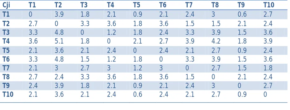
Now, the values Cji for the formation of a timing diagram which gives the response time for the given permutations of Tj and Ti are calculated using following formula:

Cji=( End index of i – Start index of j )*0.3+ Transfer Time of j

The values of Cji for the given permutations of Tj and Ti are as follows

Table II Service Table

level Tid At Sb Eb Bs AET Dl Tt

8 T1 11 5 7 3 4.5 20 1.8

6 T2 8 0 2 3 4.5 17 1.8

2 T3 1 9 10 2 3 7 1.2

5 T4 4 10 11 2 3 10 1.2

1 T5 0 6 6 1 1.5 3 0.6

9 T6 13 8 10 3 4.5 22 1.8

4 T7 0 3 4 2 3 6 1.2

10 T8 20 1 2 2 3 26 1.2

3 T9 1 7 7 1 1.5 4 0.6

7 T10 3 4 6 3 4.5 12 1.8

Cji T1 T2 T3 T4 T5 T6 T7 T8 T9 T10

T1 0 3.9 1.8 2.1 0.9 2.1 2.4 3 0.6 2.7

T2 2.7 0 3.3 3.6 1.8 3.6 1.5 1.5 2.1 2.4

T3 3.3 4.8 0 1.2 1.8 2.4 3.3 3.9 1.5 3.6

T4 3.6 5.1 1.8 0 2.1 2.7 3.9 4.2 1.8 3.9

T5 2.1 3.6 2.1 2.4 0 2.4 2.1 2.7 0.9 2.4

T6 3.3 4.8 1.5 1.2 1.8 0 3.3 3.9 1.5 3.6

T7 2.1 3 2.7 3 1.2 3 0 2.7 1.5 1.8

T8 2.7 2.4 3.3 3.6 1.8 3.6 1.5 0 2.1 2.4

T9 2.4 3.9 1.8 2.1 0.9 2.1 2.4 3 0 2.7

(6)

782 PERFORMANCE EVALUATION

A. MDTS (MULTI-DYNAMIC TRANS SCHEDULING) Algorithm

The working of MDTS algorithm is explained below:

1 Transactions are separated into three levels by type, that is, hard real-time transaction (HT), soft real-time transaction (ST), non-real-time transaction (NT). Their priorities are defined as: Prio (HT)>Prio (ST)>Prio (NT). Then, different kinds of transactions use different scheduling policies to assign priorities.

2 Lowest priority to the non-real time transaction.Here one transaction is consider for NT

3 Initially we assign the level no. to each transaction Randomly

4 According to level no. we decide which is HRT, SRT and Non-Real Time and

then assign priority to each transaction.

5 For hard transaction

Pi = (α * D + (1-α) * S)

Where,

S= de-(t0 + E-P)

D=de-t0

6 For soft transaction

Pi = S

Where,

S= de-(t0 + E-P)

7 According to priority finally schedule the transactions.

Now we apply MDTS algorithm for scheduling the transaction set in the above example as follows:

(7)

783 Level no. 1,2,3,4 are the hard real time transaction i.e. T5,T3,T9,T7

Level no 5.6,7,8,9 are the soft real time transaction i.e. T4,T2,T10,T1,T6

Level no 10 is the non-real time transaction i.e. T8

 Calculate the priority of Hard transaction as follows:

S= de-(t0 + E-P)

S(T5)=[3-(0+1.5)]=1.5

S(T3)=[7-(0+3)]=-4

S(T9)=[4-(0+1.5)]=2.5

S(T7)=[6-(0+3)]=3

Pi = (α * D + (1-α) * S)

P(T5)=0.2*3+(1-0.2)*1.5

=1.8

Service time for T5= IDHP-start block of previous*0.3+ Transfer Time of T5 =0.6

P(T3)=0.2*7+(1-0.2)*4 =4.6

P(T9)=0.2*4+(1-0.2)*2.5=2.8

P(T7)=0.2*6+(1-0.2)*3 =3

C5,7=(6-3)*0.3+1.2=2.1

Similarly,

C7,3=(4-9)*0.3+1.2=2.7

C3,9=(10-7)*0.3+0.6=1.5

 Calculate the priority of soft transaction as follows:

S= de-(t0 + E-P)

(8)

784 S(T2)=[17-(6.9+4.5)]=5.6

S(T10)=[12-(6.9+4.5)]=0.6

S(T1)=[20-(6.9+4.5)]=8.6

S(T6)=[22-(6.9+4.5)]=10.6

C9,4=(7-10)*0.3+1.2=2.1

C4,2=(11-0)*0.3+1.8=5.1

C2,10=(2-4)*0.3+1.8=2.4

C10,1=(6-5)*0.3+1.8=2.1

C1,6=(7-8)*0.3+1.8=2.1

C6,8=(10-1)*0.3+1.2=3.9

After calculations, the values Cji for all the formation of a timing diagram which gives the response time for the given permutations of Tj and Ti are used for schedule along with the number of successful transactions

Fig.1. MDTS Schedule

B. Proposed Approach based on MDTS and G-EDF Algorithms

T7

T5 T3 T9 T4 T2 T1 T6 T8

HIT=8 MISS=2

Total Response time =24.6

0.6 2.7 5.4 6.9 9 14.1 16.5 18.6 20.7 24.6

Response time

3 6 7 4 10 17 12 20 22 26 deadline

(9)

785 Here, transactions are divided into three groups HT, ST and NT same as in MDTS except that before giving service to the grouped transactions, G-EDF algorithm is applied to further divide them into groups. And then transactions are served considering highest priority group first.

The working of proposed algorithm based on MDTS and G-EDF algorithms is explained below:

1. Transactions are separated into three levels by type, that is, hard real-time transaction (HT), soft real-time transaction (ST), non-real-time transaction (NT). Their priorities are defined as: Prio (HT)>Prio (ST)>Prio (NT). Then, different kinds of transactions use different scheduling policies to assign priorities.

2. Lowest priority to the non-real time transaction. Here one transaction is consider for NT

3. Initially we assign the level no. to each transaction Randomly

4. According to level no. we decide which is HRT, SRT and Non-Real Time and then assign priority to each transaction.

5. Apply G-EDF on HT and ST groups and schedule the transactions considering highest priority group first.

6. For hard transaction

Pi = (α * D + (1-α) * S)

Where,

S= de-(t0 + E-P)

D=de-t0

7. For soft transaction

Pi = S

Where,

S= de-(t0 + E-P)

8. According to priority finally schedule the transactions.

(10)

786 Using G-EDF algorithm transactions are divided into groups as follows:

Consider the following set of transactions with their deadlines:

EDF SCHEDULE

Transactions(Ti): T3 T1 T6 T5 T4 T2

Deadlines(Di): 3 6 7 9 16 22

For formation of groups G-EDF uses the factor called as Gr-Group range factor that defines the range of number of transactions that can be included in a group. Here we will take Gr=0.5.

D1=3 i.e. first transactions deadline……

g-EDF GROUPS

For G1 D1*Gr=3*0.5=1.5

G1= {T3} for T1 as 6-3<=1.5 is false so it must be in next group

For G2 D2*Gr=6*0.5=3

G2= {T1, T6 | 7-6<=3,

T5 | 9-6<=3} for T4 as 16-6<=3 is false so it must be in next group

For G3 D5*Gr=16*0.5=8

G3= {T4,

T2 |22-16<=8 }

Now we apply the proposed algorithm (MDTS+G-EDF algorithm )for scheduling the transaction set in the above example as follows:

1. Assign level no to each transaction

Level no. 1,2,3,4 are the hard real time transaction i.e. T5,T3,T9,T7

Level no 5.6,7,8,9 are the soft real time transaction i.e. T4,T2,T10,T1,T6

(11)

787 2. Applying g-EDF on hard transaction and soft transaction

For hard transaction:-

T5 T3 T9 T7

D1=3 D2=7 D3=4 D4=6

EDF SCHEDULE

T5 T9 T7 T3

D1=3 D2=4 D3=6 D4=7

Gr=0.5 D1=3 i.e. first transactions deadline……

g-EDF GROUPS

For G1 D1*Gr=3*0.5=1.5

HG1= {T5,T9 | 4-3<=1.5}for T7 as 6-3<=1.5 is False so it must be in next group.

For G2 D3*Gr=6*0.5=3

HG2= {T7, T3 | 7-6<=3}

For soft transaction:-

T4 T2 T10 T1 T6

D1=10 D2=17 D3=12 D4=20 D5=22

EDF SCHEDULE

T4 T10 T2 T1 T6

D1=10 D2=12 D3=17 D4=20 D5=22

Gr=0.5 D1=10 i.e. first transactions deadline……

g-EDF GROUPS

For G1 D1*Gr=10*0.5=5

(12)

788 For G2 D3*Gr=17*0.5=8.5

SG2= {T2,T1| 20-17<=8.5,

T6 | 22-17<=8.5}

3. Calculate the priority of Hard transaction as follows:

S= de-(t0 + E-P)

S(T5)=[3-(0+1.5)]=1.5

Pi = (α * D + (1-α) * S)

P(T5)=0.2*3+(1-0.2)*1.5

=1.8

Service time for T5= IDHP-start block of previous*0.3+ Transfer Time of T5 =0.6

S(T7)=[6-(0.6+3)]=2.4

D(T7)=6-0.6=5.4

P(T7)= 0.2*5.4+(1-0.2)*2.4=3

C5,7=(6-3)*0.3+1.2=2.1

Similarly

S(T9)=[4-(2.7+1.5)]=0.2

D=4-2.7=1.3

P(T9)=1.54

C7,9=|(4-7)|*0.3+0.6=1.5

S(T3)=[7-(4.2+3)]=-0.8

D(T3)=2.8

(13)

789 C9,3=|(7-9)|*0.3+1.2=1.8

Similarly for soft transaction

S(T4)=[10-(6+3)]=1

S(T10)=[12-(6+4.5)]=1.5

C3,4=|(10-10)|*0.3+1.2=1.2

C4,10=|(11-4)|*0.3+1.8=3.9

S(T2)=[17-(11.1+4.5)]=1.4

S(T1)=[20-(11.1+4.5)]=4.4

S(T6)=[22-(11.1+4.5)]=6.4

C10,2=|(6-0)|*0.3+1.8=3.6

C2,1=|(2-5)|*0.3+1.8=2.7

C1,6=|(7-8)|*0.3+1.8=2.1

C6,8=|(10-1)|*0.3+1.2=3.9

After calculations, the values Cji for all the permutations of Tj and Ti are used for formation of a timing diagram which gives the response time for the given schedule along with the number of successful transactions.

Fig.2. MDTS Schedule using g-EDF Algorithm

T7 T7

T5 T9 T3 T10 T2 T1 T6 T8

T5 T4

HIT=9 MISS=1

Total Response time=24.4

0.6 2.7 4.2 6 7.2 11.1 14.7 17.4 20.5 24.4

Response time 3 6 4 7 10 12 17 20 22 26 deadline

(14)

790 III. PERFORMANCE EVALUATION GRAPH

In this section, we compared MDTS scheduling algorithm with our proposed approach which is a combination of MDTS and G-EDF algorithms. We have used number of hit transactions as performance measures to evaluate the performance. The MDTS scheduling algorithm using G-EDF is more efficient as compared to MDTS scheduling algorithm yielding higher number of hit transactions. Following graphs shows this performance evaluation.

Fig.3. Performance graph

IV. CONCLUSION

In this paper, we have illustrated the scheduling of real-time transactions using MDTS algorithm and our proposed approach which is a combination of MDTS and G-EDF algorithms. In MDTS, transactions are separated into three levels by types, that are hard real-time transaction (HT), soft real-time transaction(ST), non-real-time transaction (NT). Their priorities are defined as: Priority (HT)> Priority (ST)> Priority (NT). Then, transactions in different groups use different scheduling policies to assign priorities.

In our proposed approach, transactions are divided into three groups HT, ST and NT same as in MDTS except that before giving service to the grouped transactions, G-EDF algorithm is applied to further divide them into groups. And then transactions are served considering highest priority group first.

Then we compared MDTS scheduling algorithm with our proposed approach and used number of hit transactions as performance measures to evaluate the performance. The MDTS scheduling algorithm using G-EDF is more efficient as compared to MDTS scheduling algorithm yielding higher number of hit transactions.

7.5 8 8.5 9 9.5

MDTS Proposed

Approach Number of Hit

(15)

791

REFERENCES

1. Abbott, A. and H. Garcia-Molina, “Scheduling Real-time Transactions: a Performance Evaluation”, Proceedings of the 14th VLDB Conference, 1988.

2. Jayant R. Haritsa, MironLivny, Michael J. Carey, “ Earliest Deadline Scheduling for Real-Time Database Systems”National Science foundatiaou under grantIRI-8657323.

3. Ben Kao and Hector Garcia-Molina, “Ovierview of Real-Time Database System” PrinctonUniversity,Princton NJ 08544 USA,Standford University,Standford,CA,94305,USA(1991)

4. C. Liu, J.W. Layland, “Scheduling Algorithms for Multiprogramming in a Hard Real-Time Environment,” Journal. ACM, pp. 104-112,Jan. 1973.

5. Alma Riska, Erik Riedel, Sami Iren “Adaptive disk scheduling for overload management” Proceedings of the First International Conference on the Quantitative Evaluation of Systems (QEST’04) 0-7695-2185-1/04 $ 20.00 IEEE.

6. Saud A. Aldarmi, “Real-Time Database Systems: Concepts and Design”Department of Computer Science The University of York April 1998

7. S.Y.Amdani “Comparison of Earliest Deadline with Adaptive Earliest Deadline Algorithm” International Conference on Global Technology Initiatives vol. no.1 ISBN 978-93-5067-450-5

8. S.Y. Amdani, M.S. Ali “An Overview of Real-Time Disk Scheduling Algorithms.” International Journal on Emerging Technologies 2(1): 126-130(2011)

9. S. Y. Amdani and M. S. Ali, “An Improved Group-EDF: A Real-Time Disk Scheduling Algorithm.” International Journal of Computer Theory and Engineering, Vol. 5, No. 6, December 2013