Kinematic control of extreme jump angles in the red legged running frog, Kassina maculata

RESEARCH ARTICLE

Kinematic control of extreme jump angles in the red-legged

running frog,

Kassina maculata

Christopher Thomas Richards*, Laura Beatriz Porro and Amber Jade Collings

ABSTRACT

The kinematic flexibility of frog hindlimbs enables multiple locomotor modes within a single species. Prior work has extensively explored maximum performance capacity in frogs; however, the mechanisms by which anurans modulate performance within locomotor modes remain unclear. We explored how Kassina maculata, a species known for both running and jumping abilities, modulates take-off angle from horizontal to nearly vertical. Specifically, how do 3D motions of leg segments coordinate to move the centre of mass (COM) upwards and forwards? How do joint rotations modulate jump angle? High-speed video was used to quantify 3D joint angles and their respective rotation axis vectors. Inverse kinematics was used to determine how hip, knee and ankle rotations contribute to components of COM motion. Independent of take-off angle, leg segment retraction (rearward rotation) was twofold greater than adduction (downward rotation). Additionally, the joint rotation axis vectors reoriented through time, suggesting dynamic shifts in relative roles of joints. We found two hypothetical mechanisms for increasing take-off angle. Firstly, greater knee and ankle excursion increased shank adduction, elevating the COM. Secondly, during the steepest jumps, the body rotated rapidly backwards to redirect the COM velocity. This rotation was not caused by pelvic angle extension, but rather by kinematic transmission from leg segments via reorientation of the joint rotation axes. We propose thatK. maculatauses proximal leg retraction as the principal kinematic drive while dynamically tuning jump trajectory by knee and ankle joint modulation.

KEY WORDS: Frogs, Jumping, Kinematics, Inverse kinematics, Kassina

INTRODUCTION

The physics of jumping seem simple. Small vertebrates such as frogs and lizards tune their performance by shifting their take-off velocity and angle (Marsh, 1994; Toro et al., 2004). While this 2D view has expanded our understanding of the musculoskeletal system (Galantis and Woledge, 2003; Roberts and Marsh, 2003; Aerts, 1998; Aerts and Nauwelaerts, 2009), it does not fully explain the control of performance. As a jumping frog traces a simple path along the vertical plane, how do the elaborate 3D leg rotations (Nauwelaerts and Aerts, 2003; Astley and Roberts, 2014) act to carry the body upward and forward? Despite recent advances in frog biomechanics (Azizi and Roberts, 2010; Astley and Roberts, 2011, 2014), no study has yet explained how 3D multi-joint kinematics

resolve into a smooth planar body motion. Furthermore, how frogs modulate joint rotations to vary take-off angle remains unclear. The present study addresses how limb joint rotations modulate trajectory in jumping frogs.

Determining how jumpers modulate limb kinematics is a step towards a broader understanding of vertebrate limb mutli-functionality. Using frog pelvic anatomy as an example, a single

frog’s ability to perform multiple behaviours (e.g. jumping versus

walking) is a classic example linking skeletal morphology (Emerson, 1979; Reilly and Jorgensen, 2011) and musculature (Emerson and De Jongh, 1980) to locomotor variability; less understood is how muscles shift their control of limb motions across different modes of locomotion. Recent evidence suggests that variations between swimming versus jumping kinematics are not strongly dependent on muscle activation patterns. Rather, kinematic differences largely emerge from differences in the fluid versus solid substrates (Nauwelaerts and Aerts, 2003; Aerts and Nauwelaerts, 2009), despite similar muscle firing patterns (Emerson and De Jongh, 1980; Kamel et al., 1996; Gillis and Biewener, 2000;

d’Avella and Bizzi, 2005). In contrast, limb motions within

terrestrial modes of locomotion (walking, climbing, jumping, etc.) may be dictated by varied coordination among multi-articular leg muscles to modulate the force direction of the foot (Lombard and Abbott, 1907; Kargo and Rome, 2002). Yet, even with knowledge of how limb muscles are recruited during jumping (Emerson and De Jongh, 1980; Kamel et al., 1996; Gillis and Biewener, 2000; Gillis, 2007), we currently cannot resolve which muscles are the drivers for behavioural variation. For example, it is difficult to speculate which muscles are differentially recruited when pushing the leg rearward during walking (Barclay, 1946; Ahn et al., 2004) versus laterally for burrowing (Emerson, 1976) without knowing how individual leg joints contribute to the 3D components of overall limb motion.

In light of the complexity of 3D kinematics, how can we resolve individual joint contributions to limb motion? As an alternative to standard 3D kinematics (e.g. Euler angles), a simplified axis-angle approach may provide clarity while facilitating calculations. Briefly,

a scalar ‘3D extension’angle (θ) is defined for each joint as the

shortest angle between adjacent segments. More precisely, θ is

simply the 2D angle within the plane defined by two adjacent segments at a moment in time. To address the influence of 3D extension on body movement, additional information is required: the orientation of the plane itself must be calculated via its normal,

n, i.e. the instantaneous axis of joint rotation (Fig. 1). For simplicity,

we describe the instantaneous orientation of each joint by the angle

(φ) of nwith respect to the vertical (see Materials and methods).

Thus, the putative role of any given joint can be assessed by two

angles: θis the magnitude of motion and φ dictates how a limb

segment moves relative to the body. For any given small change in

3D extension (Δθ),φ≈90 deg suggests that 3D extension thrusts the

body forward (Fig. 1A) whereasφ≈0 deg suggests thatΔθelevates

(Fig. 1B).

Received 3 June 2016; Accepted 3 March 2017

Department of Comparative Biomedical Sciences, The Royal Veterinary College, Hawkshead Lane, Hatfield AL9 7TA, UK.

*Author for correspondence ([email protected])

C.T.R., 0000-0002-1908-3577

Journal

of

Experimental

Armed with the above framework for characterizing joint functions, the present study addresses vertical versus horizontal jumping as a subset of frog behavioural diversity. We propose a hypothetical mechanism by which frog joints influence the

instantaneous body pitch angle (ψ) to control take-off angle

(ψtake-off; Fig. 1). Given that frogs push their body upwards to

reach a‘preparation angle’during the first phase of jumps (Wang

et al., 2014), we similarly expect the limb joint axes to reach a‘joint

preparation angle’enabling frogs to aim for a steep versus shallow

jump. Specifically, we expect the rotation axes of the hip, knee and ankle to be approximately parallel such that leg segments move

within the same plane (i.e. the ‘extension plane’). Thus, we

hypothesize two mechanisms to modulateψ: (1) adjusting the initial

leg joint configuration to set the degree of inclination of the extension plane during the preparation phase (Fig. 1C) and (2) adjusting the angle of the sacroiliac joint to tilt the body upwards about the pelvis (Emerson and De Jongh, 1980; Jenkins and Shubin, 2010).

An ideal model for the present study is Kassina maculata

Duméril 1853 (African running frogs), which are grass- and reed-dwelling frogs (Wendy and Channing, 1983) that jump between perches (C.T.R., L.B.P., personal observations) as well as upwards to escape into overhanging tree leaves when frightened (Loveridge, 1976). We used high-speed video and inverse kinematics analysis to determine whether limb segment motions and joint axes of rotation predict jump angle.

MATERIALS AND METHODS Animals

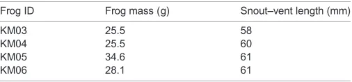
Adult K. maculata frogs (28.4±3.7 g body mass; 60.0±1.2 mm

snout–vent length;N=4; Table 1) were obtained from Amey Zoo

(Hempstead, UK). Animals were housed in terraria at the Royal Veterinary College at 25°C under a 12 h:12 h light:dark cycle and were fed two to three times weekly.

Experimental procedures

Small plastic circular markers (∼5 mm diameter) were cut from thin

plastic sheets (∼0.25 mm thick) using a screw punch (Nonaka Mfg.

Co. Ltd., Japan) with a 5 mm hollow point drill bit, and then painted with white correction fluid. Markers were placed on anatomical landmarks on the body (head, vent) and left leg [hip, knee, ankle, tarsometatarsal (TMT) joint] using cyanoacrylate adhesive. Frogs were then stimulated to jump while filmed from two orthogonal views at 250 Hz, 1/1500 shutter speed using a pair of Photron SA3 high-speed video cameras (Photron Ltd, Tokyo, Japan). An inclined mirror was used to obtain a third view to track landmarks on the body and limb simultaneously. Prior to each jump, frogs were placed at the same starting position on a small force platform (see Porro et al., 2017). A range of jump angles were elicited by consistently varying the height of the frog box using pre-cut wood blocks of pre-determined thickness. Trials in which the frog turned

Table 1. Experimental summary, including information on subjects and trials

Frog ID Frog mass (g) Snout_–vent length (mm)

KM03 25.5 58

KM04 25.5 60

KM05 34.6 61

KM06 28.1 61

List of symbols and abbreviations Ai instantaneous rotation axis for theith joint

Âi instantaneous rotation axis for theith joint expressed as a unit vector

B body axis vector COM centre of mass d_ψ/dt body rotational velocity IK inverse kinematics J full Jacobian matrix

J′ pseudoinverse of the Jacobian matrix

JRi rotational subset of Jacobian matrix for theith joint JTi translational subset of Jacobian matrix for theith joint M matrix ofxyzcoordinates for kinematics landmarks in the

camera reference frame

M_′ matrix ofxyzcoordinates for kinematics landmarks rotated to the trackway reference frame

PF proximal foot

Pi xyzcoordinates of theith point (landmark) on the body or limb R 3×3 rotation matrix to correct for yaw angle (_α)

tc contact time

TMT tarsometatarsal ( joint)

vtarget target velocity vector for inverse kinematics analysis

Y globaly-axis vector

α body yaw angle (angle aboutz-axis)

θ ‘3D’joint angle

ψ take-off angle (see Fig. 1)

φi angle between the instantaneous rotation axis of theith joint and horizontal (see Fig. 1)

Δq vector of incremental change in joint 3D angles

A

B

C

D

Knee

Ankle

TMT Velevation

Vthrust

Hip y

z

z

x y x

x

z

y

ψ=45 deg ψ=0 deg ψ=90 deg

φ=45 deg

φ=0 deg φ=90 deg

Fig. 1. Schematic view of a frog jump.(A) Top view showing bones in the horizontal plane with rotation axes (φ) oriented vertically resulting in horizontal jumps (ψ=0). (B) Side view showing bones in the sagittal plane with rotation axes oriented horizontally to produce a vertical jump (_ψ=90). (C) Three-dimensional view showing rotation axes at 45 deg within a hypothetical ‘extension plane’(white box) within which the bones rotate to determine the inclination of the take-off angle. Extension of the joints in this configuration results in both forward (Vthrust) and upward velocity (Velevation). (D) Rear view

showing how joint rotation axes need not be tied to the extension plane. For example, the ankle orientation can shift to a different orientation (blue lines) independent of the orientation of the knee. Note that A and B are extreme cases for illustrative purposes only and are not actually observed in frog jumping.

Journal

of

Experimental

during the jump (i.e. asymmetric leg extension) were discarded. All experimental procedures were approved by the UK Home Office (License 70/8242).

Data processing

Video data from three views were calibrated using direct linear

transformation and landmarks were‘digitized’toXYZcoordinates

using open source script (Hedrick, 2008) run in MATLAB (MathWorks, Natick, MA, USA). All subsequent data processing

and analysis was performed in Mathematica (Wolfram,

Hanborough, UK).XYZcoordinate data were filtered by a

second-order lowpass Butterworth filter using a 25 Hz cut-off frequency to smooth video tracking error.

Calculation of 3D joint angles and segment orientations

The camera views defined a right-handed global reference frame

with the y-axis pointing forward along the trackway, the x-axis

pointing right and thez-axis pointing up (Fig. 1). For each video

frame, digitization of seven landmarks yielded a 7×3 matrix,M(i.e.

sevenxyzpoints). Although only straight jumps were included in

analysis, frogs rarely initiated their jumps exactly parallel with the trackway axis. Occasionally, frogs began with an initial angle within 10 deg of the trackway axis, but carried on moving along the same direction (i.e. frogs did not turn during the included jumps). Thus,

for every video frame,Mwas rotated (M′) to align the points along

the axis of the jump, effectively moving the camera to align with the forward axis of the jump (see Appendix 1).

Landmarks placed on the leg were used as a proxy for rigid body motion of the limb segments. Leg segment angles were calculated using local reference frames anchored at joint centres of rotation (assumed to coincide with landmark positions) as follows. For each

joint, the global Cartesian x-y-zaxes were anchored at the given

joint centre.XYZcoordinates of the distal tips of the leg segments

(thigh, shank, and proximal foot) were converted to spherical polar

coordinates (i.e. [x, y, z]→[r, θxy, θz]). For example, the thigh

segment angle was calculated using the hip as the origin and the

distal tip of the segment (i.e. knee) as the point of interest,P, in the

hip local reference frame. Converting P into spherical polar

coordinates yields a length (r=segment length) and two angles:

(1) the angleθxyin the horizontalXYplane (retraction) and (2) the

angleθzwith respect to the global vertical axis (adduction). Note

that for convenience, we offsetθzby−90 deg so that angles could be

based from the horizontal (i.e. a segment oriented horizontally has an adduction angle of 0 deg; see Fig. 1).

For joint motions, the axis-angle convention was used. The rows

ofM′containedxyzcoordinates for the snout, vent, hip, knee, ankle

and TMT landmarks (Ps,Pv,Ph,Pk,Pa,Pt, respectively), which were

used as proxies for joint centres of rotation as well as end points of the thigh, shank and proximal foot (PF) segments. Thus, subtracting adjacent points gave segment vectors used for approximating

instantaneous 3D rotation axes (A) for the hip, knee and ankle:

Ah¼ ðPsPvÞ ðPkPhÞ; ð1Þ

Ak¼ ðPhPkÞ ðPaPkÞ; ð2Þ

Aa¼ ðPkPaÞ ðPtPaÞ; ð3Þ

whereAh,AkandAaare rotation axes of the hip, knee and ankle,

respectively, and × denotes the cross-product. All axes were converted to unit vectors by dividing them by their magnitude (e.g.

Âh=Ah/||Ah||, etc.) before calculating the vertical orientation angle

(φ) with respect to horizontal (in radians):

fh¼cos1ðA^h;zÞ p=2; ð4Þ

(and similarly for the knee and ankle joints), where Âh,z is the

z-coordinate of the normalized hip rotation axis vector. Note that

theXYplane (horizontal) was defined here as 0 deg. Note also that

because the knee rotation axis direction is opposite that of the hip and ankle, the knee orientation angle was negated.

Time series analysis

To statistically compare temporal patterns among trials, time series

data were normalized by percent of jump contact time

(tc=tend−tstart), where tend was defined as the final video frame where the foot is seen in contact with the surface. Because jumps are not periodic behaviours, we used the body centre of mass (COM) motion to mark the onset of jumps. COM resultant velocity was estimated as the velocity of a body landmark near the hip. For each trial, the time-varying magnitude of the COM resultant velocity vector was fit to a six-order polynomial. The time value for the first zero crossing (i.e. start of body velocity) of the polynomial equation

was used as an estimate oftstart. Translational velocity values are

reported in body lengths s−1_{(absolute velocity/snout–vent length).}

Inverse kinematics analysis

To explore the posture-dependent influence of hip, knee and ankle extension on COM motion, we used inverse kinematics (IK) to

hypothetically‘back-calculate’changes in 3D extension angles (q)

required given a target body velocity angle (ψ), i.e.:

c!DCOMzy!Dq; ð5Þ

where ΔCOMzyis the change in the position of the body in the

vertical plane. Specifically, we used IK to address how frogs may modulate the angle of their body velocity vector (thus influencing

the instantaneous body velocity angle, ψ, and take-off angle,

ψtake-off) by adjusting hip, knee and ankle joint angles to achieve a desired trajectory at any given instant in time. Similarly, IK can predict changes in joint angles required for a change in body rotational velocity:

dc

dt !Dq: ð6Þ

To explain more thoroughly, IK analysis relates changes in joint

angles (q) to the linear velocity of the limb endpoint. In a robotic

arm, for example, IK computes the joint angles necessary to achieve a desired linear velocity of the hand towards a target. For a frog limb

at a given posture, one can calculate a small change (Δq) required to

move the head in a given direction. Importantly, IK does not account for masses and moments-of-inertia of the limb segments, hence it ignores the required forces/torques in the system. Rather, IK assumes that the muscles (or electric motors in a robot) can produce sufficient force (or torque) to achieve the desired kinematics. Regardless, IK can be used as a modelling tool to hypothetically address how a frog might extend its joints to adjust its instantaneous

body velocity (hence body angle,ψ; Fig. 1) and its rate of change

(hence dψ/dt). Because of the many possible ways in which a frog

limb can move, there likewise exist many solutions forΔqto achieve

a desired instantaneous ψ or dψ/dt. Implicitly, IK calculates the

minimal requiredΔq, and thus reveals a plausible hypothesis for

how joint rotations might influence COM motion. The steps to compute joint angle changes in response to a hypothetical change in

ψare as follows.

Journal

of

Experimental

First, a target body velocity vector is calculated based on the reference frame currently used by rotating an arbitrary point along

they-axis (cranio-caudal axis; Fig. 1) about thex-axis by an angleψ:

1 0 0

0 cosðcÞ sinðcÞ

0 sinðcÞ cosðcÞ

2 4

3 5 01

0

2 4

3

5_¼vtarget: ð7Þ

Second,Δqis found by matrix multiplication:

Dq¼J0Tvtarget¼

Duankle

Duknee

Duhip 2 4

3

5_{; ð}8Þ

wherevtargetis a column vector ofx,y,zcoordinates,Δθare changes

in hip, knee and ankle 3D extension angles andJ′Tis a 3×3 matrix

computed as the pseudoinverse of the translational portion of a modified Jacobian matrix (i.e. a matrix that converts between joint angular velocities and end-of-limb linear velocity; see Appendix 2). With simple geometry (e.g. a single bone rotating about a hinge-like joint), one can easily see the relationship between angular rotation and linear excursion at the tip of the limb. However, with multi-joint systems (such as robotic arms, frog legs, etc.), the cumulative motions caused by in-series joints can only be known through messy calculations. Consequently, how individual joint rotations contribute to motion at the end of the limb (e.g. the hand of a robotic arm or the body of a frog) is not obvious. To address this, Jacobian matrices are used in kinematics and dynamics analysis because they allow one to translate joint movements into end-of-limb movements and vice versa.

Similarly, the calculatedΔqrequired for a hypothetical change in

dψ/dtis:

Dq¼J0 vtarget

dc=dttarget

¼ DuDuankleknee

Duhip 2 4

3

5_{; ð}9Þ

whereJ′is the 6×3 pseudoinverse of the modified Jacobian matrix

(see Appendix 2). For the present analysis,vtargetwas first selected

usingψ=1 rad (≈60 deg) to represent the steep jump trials (Eqn 7).

Then,dψ/dttargetwas determined from theΔqdue to the selected

vtarget.

Statistics

Descriptive statistics were performed on data from n=50 jumps

pooled overN=4 animals. Data were arbitrarily divided into three

categories based on jump take-off angle (see above) for data plotting and descriptive statistics. After dividing jump angle values into quantiles, low jumps were classified as below the first quantile, middle jumps between the first and third quantiles and high jumps above third quantile. ANCOVAs were used to compare several separate performance variables for their influence on increasing

jump angle. A significance threshold ofP=0.05 was used for the

regression component ( jump angle versus performance variable), individual effects among frogs (frog) as well as interactions (frog×jump angle). Statistical analyses were performed in Mathematica.

RESULTS

Jump performance and descriptive kinematics

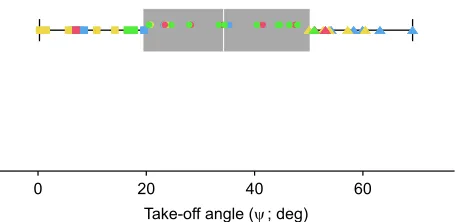
Jump performance varied widely among trials, with take-off angles ranging from 0.27 deg to nearly 70 deg pooled across all frogs. The average minimum jump angle (minimum angle averaged across all frogs) was 7.61±6.68 deg and the maximum was 58.43±8.24 deg,

while peak resultant velocities ranged from 16.49±3.64 to 31.47±

3.27 body lengths s−1 _{(mean±s.d., N=4 frogs; Fig. 2). The}

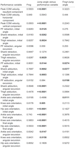
distribution among pooled jump angle data suggested data partitioning into low (<20 deg) versus high jumps (>50 deg) with the remainder designated as middle jumps (see Materials and methods). Each individual frog represented nearly the entire performance range (see Table S1) and there was no observed effect of individual frog on the performance variables measured (Table 2).

Despite variation in jump angle and take-off velocities, limb and body kinematics were qualitatively similar. The sacroiliac angle change was statistically significant, but modest in magnitude and

rate compared with‘3D extension’angles of hip, knee and ankle

joints (Fig. 3B), which propelled frogs toward peak translational

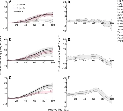
velocity by the time of take-off (Fig. 4A–C). At take-off, the

resultant COM velocity increased significantly with jump angle

(ANCOVA,P<0.0001) as a function, not surprisingly, of the rising

vertical component magnitude (Table 2, Table S1). Surprisingly, despite the lack of strong sacroiliac rotation, steep jumps were marked by rapid pitching rotational velocity of the body segment

(dψ/dt) that was less apparent for low and intermediate jumps

(Fig. 4D–F).

Leg segment kinematics

Segment orientations for the thigh, shank and PF were calculated in local joint reference frames anchored at the hip, knee and ankle, respectively (see Materials and methods). Retraction (about the

local Z-axis) and adduction (about the local Y-axis) carried the

thigh, shank and PF segments backward and downward. Seen from

dorsal (‘top’) view, segments mainly retracted as the distal ends of

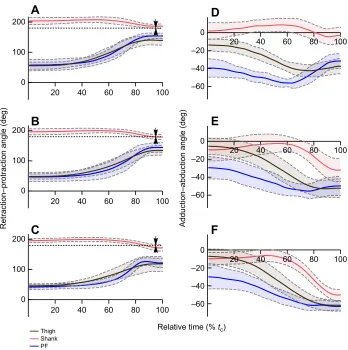
limb segments moved posteriorly (see Figs 1 and 3). Segment retraction patterns were qualitatively similar across jump angle. Although limb segments began at smaller retraction angles (i.e.

more ‘flexed’ posture) for shallower jumps, jump angle was

independent of total minimum–maximum angular excursion

(retraction) for all segments except for the thigh (ANCOVA; Table 2, Table S1). In all trials, the thigh and proximal foot retracted in concert causing the two to remain parallel in dorsal view as they retracted. In contrast, the shank orientation remained nearly constant

during the earliest∼80% of jumps before retracting (straightening)

slightly to align with the body midline in the final stage of take-off

(Fig. 5A–C).

Unlike the observed retraction patterns, segment adduction (downward rotation towards the ventral body midline) varied

qualitatively among segments and jump angles (Fig. 5D–F). Initial

adduction angles varied differentially among segments (ANCOVA,

0 20

Take-off angle (ψ; deg) 40 60

Fig. 2. Box and whisker plot showing the interquartile range (IQR; grey box) and median (white line) of jump angle data for_n=50 trials pooled over four animals (different colours).Low jumps (squares) fall below the median whereas high jumps (triangles) are above 1.5×IQR. The remaining represent intermediate jumps (circles).

Journal

of

Experimental

P<0.05; Table 2). More importantly, however, increasing jump angle was strongly predicted by greater thigh and shank adduction excursion (Table 2, Table S1). Most notably, average shank orientation remained nearly horizontal except for medium and steep jumps, which were marked by increasingly strong adduction

during the final∼20% of take-off time (Fig. 5F).

Joint‘3D extension’orientations

Limb segment motions were described using the axis-angle convention (see Materials and methods; Fig. 1). Briefly, the

relative orientation of two adjacent segments (e.g. thigh and shank) was defined by two parameters: the 3D extension angle (i.e. the shortest angle between two segments) and the 3D axis of rotation.

The former determines the ‘straight-line’ displacement between

joints whereas the latter determines the direction.

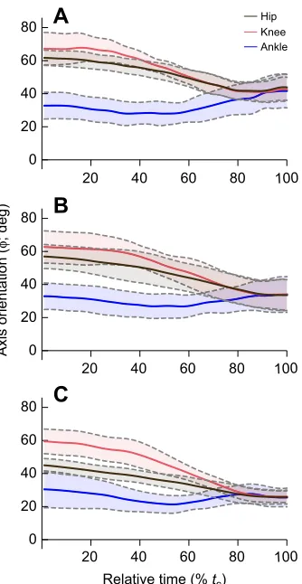
Frogs showed a similar pattern of joint orientation among jumps. Generally, joint axes were time-varying, indicating that the effects of 3D extension shifted during jumping (Fig. 6). Hip and knee

rotation axes began nearly vertical, but reoriented to ∼45 deg

throughout jump duration, suggesting a functional transition from pure retraction to retraction+adduction. In contrast, the ankle rotation axis began at a lower angle (closer to horizontal) and increased through time, signifying a shift from adduction to retraction+adduction. A striking general pattern emerged across

all jumps: during the final∼20% of jumps, hip, knee and ankle joint

axes converged towards a common angle; consequently, all hind

limb joints rapidly shifted into alignment (Figs. 3A inset, 6A–C).

Changes in axis orientations co-varied significantly with jump angle. Most notably, at higher jump angles the final orientation angles of hip, knee and ankle joints decreased significantly

(ANCOVA, P<0.0001; Table 2, Table S1). Specifically, shallow

jump angles appear to result from nearly vertical rotation axis

orientations (φcloser to 90 deg) whereas steep jumps correlated with

more horizontal orientation angles (φcloser to 0 deg; see Fig. 1A

versus B). Functionally, this shift from high orientation angles (shallow jumps) to low orientation angles (steep jumps) suggests a putative mechanism for modulating take-off angle via control of rotation axes (see Discussion). In addition to take-off kinematics, the pre-jump limb posture in the early phase of the jump was also a predictor for jump angle. For increasing jump angles, the hip and knee orientations became less vertical, suggesting an increasing bias towards vertical COM motion.

Inverse kinematics predictions of joint function

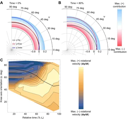
IK analysis predicted differential roles for the hip, knee and ankle joints. This analysis predicts how hypothetical extension of an individual joint might have the potential to act to move the frog at a given point in time. Near time=0%, ankle 3D extension showed potential for increasing the body velocity angle of kinematic models (Fig. 7A) whereas combined ankle and knee 3D extension showed the strongest effects late (time=80%; Fig. 7B). IK was similarly used

to model the roles of joint extension on body rotational velocity (dψ/

dt), which is partially caused by simultaneous knee 3D extension

combined with the decreasing angle of the knee rotation axis (Fig. 7C; see Discussion).

DISCUSSION

Frogs modulate jump angle by postural preparation and by dynamic modulation of joint kinematics

The present study addressed how frog joint kinematics shift to enable flexibility of jump angles. Because prior work found that forelimb preparation angle predicts take-off angle (Wang et al., 2014), we

hypothesized an analogous ‘joint preparation angle’whereby leg

joints form a ‘3D extension plane’whose inclination is preset to

determine final take-off angle (ψtake-off; Fig. 1). Additionally, we

expected sacroiliac extension to modulate take-off angle. Current findings support aspects of each hypothesis, but neither entirely. Regardless, general patterns emerged across all animals and jumps. Frog jumps were powered by limb segment retraction (rearward rotation pushing the body forward) and adduction (downward rotation elevating the body; Nauwelaerts and Aerts, 2003; Astley and

Roberts, 2014) as well as rotational pitching velocity (dψ/dt). Within

Table 2.P-values from linear mixed-model statistics for kinematics performance variables forn=50 trials overN=4 frogs

Performance variable Frog

Jump angle versus performance variable

Frog×Jump angle

Peak COM velocity, resultant component

0.5503 <<0.0001 0.3223

Peak COM velocity, horizontal component

0.849 0.0943 0.444

Peak COM velocity, vertical component

0.0503 <<0.0001 0.2243

PF retraction, initial angle

0.8283 0.0125 0.275

Shank retraction, initial angle

0.8183 0.0262 0.0598

Thigh retraction, initial angle

0.8257 0.0024 0.7842

PF retraction, angular excursion

0.8396 0.059 0.253

Shank retraction, angular excursion

0.8447 0.1274 0.2461

Thigh retraction, angular excursion

0.8287 0.0029 0.8626

PF adduction, initial angle

0.8051 0.0144 0.0274

Shank adduction, initial angle

0.7697 0.0002 0.0377

Thigh adduction, initial angle

0.7844 0.0003 0.1296

PF adduction, angular excursion

0.8152 0.084 0.0198

Shank adduction, angular excursion

0.0646 <<0.0001 0.2322

Thigh adduction, angular excursion

0.4478 <<0.0001 0.0994

Ankle axis orientation, initial angle

0.8195 0.4996 0.0111

Knee axis orientation, initial angle

0.8176 0.005 0.2113

Hip axis orientation, initial angle

0.4561 <<0.0001 0.1427

Ankle axis orientation, final angle

0.743 <<0.0001 0.3976

Knee axis orientation, final angle

0.5853 <<0.0001 0.4015

Hip axis orientation, final angle

0.5933 <<0.0001 0.5515

Ankle axis orientation, angular excursion

0.8342 0.0147 0.4191

Knee axis orientation, angular excursion

0.8431 0.0158 0.8502

Hip axis orientation, angular excursion

0.8552 0.1809 0.5272

COM, centre of mass; PF, proximal foot. Note that angular

excursion=maximum value−minimum value. Values in bold are significant at the 0.05 level.

Journal

of

Experimental

this observed behavioural variation, we sought joint kinematic evidence explaining two mechanisms: (1) how do leg joints

influence body velocity angle (ψ) via relative amounts of forward

thrust versus elevation; and (2) how do joints influence upward

pitching rotational velocity of the body (dψ/dt)? Our three key

findings are as follows. Firstly, although we found thatK. maculata

150 Snout

Rear view

A

B

φ SI

z

x

Knee Foot Hip

Ankle TMT

100

3D joint angle (deg)

50

0.05 0.10 Time (s)

0.15 0.20

Fig. 3. Three-dimensional leg kinematics from an example jump.(A) Three-dimensional view and rear view (inset) schematic showing kinematics from five key frames of an example jump. The black spheres are skin marker landmarks for the right leg and body (red), mirrored for the left (grey). Subsequent frames show right leg only, offset in space for clarity. Shaded areas are hip and ankle_‘3D extension angles_’with their respective rotation axes (blue lines), similarly labelled for the rear view (inset). For illustration, axes lengths are scaled to snout–vent length. The knee axis (dashed) is omitted from the 3D view for clarity. Note the reorientation of rotation axes as they align at the final frame. (B) Three-dimensional angles for sacroiliac (SI; green), hip (black), knee (red), ankle (blue) and TMT (orange) from the example trial in A. Note that the sacroiliac joint is not depicted in the illustrations, but is represented as a rotation axis in the horizontal plane (green, dashed line).

Relative time (% _tc) 40

A

B

C

D

E

F

Resultant

Horizontal

Vertical

30

20

10

–10

20 40 60 80 100

20 15 10 5

–10 –5

20 40 60 80 100

20 15 10 5

–10

Rotational velocity (d

ψ

/d

t

) (rad s

–1

)

–5

20 40 60 80 100

20 15 10 5

–10 –5

20 40 60 80 100 40

30

20

10

–10

T

ranslational velocity (body lengths s

–1

)

20 40 60 80 100

40

30

20

10

–10

20 40 60 80 100

Fig. 4. Translational and rotational COM velocity (see Materials and methods).Resultant (black), horizontal (red) and vertical (grey) translational velocity components are shown for low (A), intermediate (B) and high angle jumps (C), and similarly for rotational velocity (D–F), where positive versus negative values indicate pitching upwards versus downwards, respectively. Time is relative to contact time (tc; see

Materials and methods). Data are means±s.d. forn=50 trials pooled over four animals.

Journal

of

Experimental

adjust aspects of initial joint posture, jump angle does not appear to be solely predetermined by initial limb configuration. In addition to adjusting initial pose, frogs appear to dynamically modulate their leg kinematics late during jumps by adjusting shank adduction as well as the inclination of hip, knee and ankle rotation axes. Secondly, we

found evidence for a‘3D extension plane’governing take-off angle,

but only in the final 20% of jump duration as the joint rotation axes rapidly orient into alignment. The influence of this alignment is not immediately clear, but could be investigated with forward dynamics

modelling in future work. Thirdly, body rotational velocity (dψ/dt)

was negligible in low and intermediate jumps, but contributed strongly to the steepest jumps.

Regardless of jump angle, K. maculata showed stereotyped

kinematics, perhaps giving insight into the underlying

musculoskeletal mechanics of jumping. After the onset of body

motion, jumps proceeded in two phases: a slow‘preparatory’phase

followed by a fast ‘launch’ phase. Similar to ranid frogs, the

preparatory phase (roughly first∼60–80% of duration) is marked

both by forelimb contact (Wang et al., 2014) and slow acceleration of the COM (Fig. 4). In contrast, the launch phase is characterized by rapid retraction and adduction via hip, knee and ankle 3D extension (Fig. 5). Additionally, the joint axes of rotation rapidly reorient to align just before take-off (Fig. 6).

Kinematic mechanisms

Knee and ankle joints may control jump velocity angle (ψ)

The striking consistency of joint rotation patterns, even for the most extreme jump angles, suggests an underlying kinematic control

mechanism that is adjusted to vary take-off angle. To escape, arboreal frogs must achieve the correct mixture of upwards and forwards COM motion to reach a particular perch. Ideally, extension at each joint would transmit the desired combination of elevation and thrust to the body at every instant in time. More likely, however, because of the 3D posture of frogs, each joint does not necessarily move the body in a useful direction. While one joint may contribute to elevation, another joint may simultaneously act to depress the

COM. Adding to this complexity, a particular joint’s kinematic

influence depends on the instantaneous orientations of other limb segments, each varying through time. Accounting for this interdependence of joint function, IK analysis predicted time-varying function among the main leg joints. During the preparatory phase (time=0%), ankle 3D extension is predicted to be the main contributor to increased body velocity angle (Fig. 7A), which is counterintuitive given the proximal-to-distal sequence of joint extension characteristic in frog jumping (e.g. Peters et al., 1996). To explain, IK does not necessarily indicate how joints are acting, but

rather how they have the potential to act (i.e. a prediction of a joint’s

effect if it were to increase torque or extend). Although IK predicts the ankle has high potential to influence jump angle early in the jump, we are not suggesting that the ankle must extend prior to

proximal joints. IK is simply predicting that the ankle’s influence on

jump angle is high early in the jump, so that when the ankle begins

extending (in the first∼10% of the jump), it will exert a relatively

strong effect on instantaneous body angle. In contrast, combined ankle and knee 3D extension are predicted to exert the strongest effect during the launch phase (time=80%), with the knee

Relative time (% tc)

A

B

C

D

E

F

Thigh Shank PF

20 200

Retraction–protraction angle (deg) Adduction–abduction angle (deg)

0

–20

–40

–60 100

0

40 60 80 100

20 40 60 80 100

0

–20

–40

–60

20 40 80 100

0

–20

–40

–60

20 40 60 80 100 20

200

100

0

40 60 80 100

20 200

100

0

40 60 80 100

60

Fig. 5. Leg segment kinematics across a range of jump angles.Limb segment protraction–retraction angles for the low, intermediate and high angle jumps (A–C, respectively) and abduction–adduction angles (D_–F, respectively). Traces are for thigh (black), shank (red) and proximal foot (blue). The black dashed line (A–C) represents a line drawn posterior from the hip joint from which protraction_–retraction angles were referenced (see Fig. 1). Trending towards the line (arrows) denotes retraction. Thex-axis (D–F) represents the horizontal axis. Downward slopes indicate adduction. Time is relative to contact time (tc; see

Materials and methods). Data are means±s.d. forn=50 trials pooled over four animals.

Journal

of

Experimental

contribution dominating the steepest angles (Fig. 7B). From a dynamic control perspective, our model predicts that if the nervous system were aiming to elevate the body, it might increase activation to ankle extensors early in the jump followed by the addition of knee extensors later during launch. Although IK results are hypothetical,

they suggest which joint motions are most ‘kinematically

parsimonious’ for transmitting motion to the body. Thus, they

may be interpreted as control hypotheses to be tested by further experiments (e.g. electromyography).

Knee axis orientation may control body pitch velocity (dψ/dt)

In addition to the greater body elevation during the steepest jumps,

K. maculataalso rotated their body rapidly to increase body velocity angle (Fig. 4F). Given the weak rotational velocity observed at the sacroiliac joint (Fig. 3), the origin of the rapid body rotational

velocity (dψ/dt) is not clear, although the forelimbs could play a role

(Wang et al., 2014). As argued above, 3D extension at any joint influences the ratio of body thrust versus elevation. Similarly, IK can predict changes in joint angles required for a change in body

rotational velocity. Counterintuitively, IK predicts that dψ/dt is

partially caused by simultaneous knee 3D extension combined with the decreasing angle of the knee rotation axis (Fig. 7C). As the knee rotation axis tilts away from vertical (Fig. 6), the leg joints become able to pitch the body upward while elevating the COM by the

mechanism above. This can be most clearly seen during the period of greatest knee axis change coinciding with the steepest increase in

rotational velocity (time∼50 to 80%; Fig. 7C). Hypothetically, if

the knee axis fails to tilt, the joint angle changes required for a steep

jump (ψ≈60 deg) would cause abduction (upward rotation) of the

femur and shank, consequently pitching the body down. However, as the knee axis orientation tilts downward (either via femur or shank adduction; Fig. 5), 3D knee extension effectively rotates the lower limb downward to pitch the body up. More succinctly, IK suggests that COM elevation and rotation would be mutually exclusive without appropriate reorientation of the knee axis. Further forward dynamics analysis would be required to confirm whether knee axis reorientation contributes to body rotational velocity. Moreover, forward dynamics would additionally be required to assess whether the observed kinematics are most effective compared

with simulations that have been ‘optimized’ (e.g. for power

generation or efficiency).

Do extreme jump angles represent distinct locomotor tasks?

The above IK analysis offers hypothetical mechanisms by which

K. maculatamay fine-tune take-off angle over a continuous range. However, the pronounced kinematic difference of steep jumps (e.g. high rotational body velocity; Fig. 4F versus D,E) may suggest that the underlying musculoskeletal mechanics do not vary continuously with inclination. Rather, extreme high versus low take-off angles may represent two biomechanically distinct movements: vertical versus horizontal locomotion. As the legs adapt different postures to overcome varying amounts of gravitational loading, they perhaps demand different recruitment patterns within and among muscle groups. Analogously, from an ecological perspective, vertical versus horizontal versus diagonal jumps may also be interpreted as distinct locomotor behaviours. For example, vertical jumps are required for escape (Loveridge, 1976) versus diagonal jumps for

distance (Marsh, 1994) versus horizontal‘jumps’to lunge after prey

(Deban and Nishikawa, 1992). Hence, we propose that although traditional 2D models of vertical jumps have been used as a template for all jumps (e.g. Alexander, 1995; Galantis and Woledge, 2003; Aerts and Nauwelaerts, 2009), they may not be appropriate for the entire range of jumping. Future investigation would be required to determine whether vertical jumping and horizontal jumping represent two distinct behaviours.

Limitations of the study require future experiments measuring ground reaction forces and bone movements

There are two main limitations to the present study. Firstly, external landmarks were used to reconstruct body and limb motions; thus, joint centres of rotation could not be precisely located. More importantly, because each segment was only defined by a pair of skin markers, true rigid body motions (i.e. rotations about each

segment’s local reference frame) could not be calculated. Generally,

any observed‘3D extension’may stem from a combination of local

extension, adduction or long-axis rotation. However, owing to the limitations of skin marker kinematics, we cannot resolve whether an apparent downward rotation of the shank resulted from an adduction of the knee joint or internal long-axis rotation of the femur about the hip. Consequently, we can only speculate on putative contributions of extensor versus adductor versus rotator muscles to limb motion. Future use of X-ray reconstruction of moving morphology (XROMM; Brainerd et al., 2010) will be used to clarify whether adduction or internal rotation drives body elevation during jumps. Additionally, XROMM data could be used to compare a more thorough standard analysis of Euler angles with our simplified

80

A

B

C

Hip Knee Ankle

60

40

20

0

20 40 60 80 100

80

Axis orientation (

φ

; deg)

60

40

20

0

20 40 60 80 100

80

60

40

20

0

20 40

Relative time (% tc)

60 80 100

Fig. 6. Joint rotation axis orientations across a range of jump angles. Orientations of hip (black), knee (red) and ankle (blue) axes of rotation for low (A), intermediate (B) and high angle jumps (C). Angles are drawn with respect to the horizontal plane such that 0 deg is horizontal and 90 deg is vertical, indicating pure adduction/abduction or retraction/protraction, respectively. Time is relative to contact time (tc; see Materials and methods). Data are

means±s.d. forn=50 trials pooled over four animals.

Journal

of

Experimental

axis-angle analysis to better assess the full utility of current approaches.

Secondly, a pure kinematics analysis can only speculate on the functional roles of joints in the absence of further analysis of ground reaction forces and joint torque estimates. Although IK predicts potential contributions of joint motion, pure kinematics analysis

does not measure the ‘effort’required to jump, and thus cannot

disentangle how force, work and power requirements might shift as frogs aim for steeper angles (see Porro et al., 2017). Joint kinematics emerge from the balance of muscle torques and external torques from ground reaction forces. Hence, while a purely kinematic study is an important first step to investigate putative joint function, it can be misleading without further analysis. Although we report how 3D

extensions may ‘control’ either forward or upward body motion

(Fig. 7), these are hypothetical effects which must be confirmed by inverse and forward dynamics analysis. For example, without knowledge of net joint torques one cannot determine whether an apparent extension movement was controlled by active torque at that joint or produced under the influence of other joints via the ground reaction force. In another example, we interpret from IK analysis

that rotation of the knee joint axis (e.g. via knee adductors) drives the pitching motion to the body segment. However, another plausible interpretation is that active pitching of the body segment (e.g. due to thigh or pelvic musculature) transfers rotational kinetic energy to the knee joint, causing it to reorient passively. Kinematic analysis cannot discern between these possibilities without forward dynamics simulation. In the spirit of 2D models of human jumping (e.g. Bobbert and van Ingen Schenau, 1988), future use of inverse dynamics (Porro et al., 2017) combined with electromyography will lead to an integrated understanding of muscle function, 3D joint mechanics and jump performance for sprawled limb jumpers. Regardless of the limitations, kinematics analysis is an important complement to dynamics analysis: dynamics analysis resolves which joints drive limb motion, whereas kinematics analysis resolves how the motions themselves translate to coordinated behaviour.

Conclusions and interpretation

The present study usedK. maculataas a model to explore how frogs

modulate jumping performance. It is the first known study to

90 deg Time = 0%

A

C

B

75 deg

60 deg

45 deg

30 deg

15 deg

0 deg 0.2

80

60

Knee axis orientation (

φ

; deg)

40

20

20 40 60 80 100 0

–0.8 φ Hip

ψ ψ

φ Knee φ Ankle

90 deg

Time = 80% 75 deg

60 deg

45 deg

30 deg

15 deg

0 deg Max. (–) contribution

Max. (+) rotational velocity (dψ/dt)

Max. (–) rotational velocity (dψ/dt) Relative time (% tc)

Max. (+) contribution

0.2 0 –0.8

Fig. 7. Inverse kinematics (IK) predictions based on an average intermediate angle jump.Radial plots show the hypothetical influences of hip (black), knee (red) and ankle (blue) 3D extension on instantaneous body velocity angle (_ψ) for (A) 0% time and (B) 80% time. The blue-to-red gradient indicates positive-to-negative contributions. The dashed line indicates 0. Note the positive-to-negative values for the hip at time 80%–i.e. hypothetically, the hip would be required to flex to reorient the limb to angles greater than∼45 deg. (C) Influence of knee axis orientation on body rotational velocity (dψ/dt) through time. The black line indicates the mean knee axis orientation for intermediate angle jumps. Note the increase indψ/dtas the knee rotation axis orientation decreases.

Journal

of

Experimental

address how 3D leg segment kinematics leads to coordinated control of the body angle and body rotational velocity. Future studies would be required to determine whether other species employ similar mechanisms.

As frogs varied take-off angle, we found that leg segments shifted the amount of abduction/adduction relative to protraction/retraction.

These ‘3D effects’ corroborate computational evidence that 2D

planar joints are insufficient to modulate jump angle (Kargo et al., 2002). Specifically, we found two main kinematic mechanisms influencing take-off angle: (1) shank adduction (downward rotation) presumably pushed the body upward late during the launch phase, and (2) rapid rotational velocity (backward pitching) caused the body to tilt vertically, contributing to a steeper take-off. IK modelling suggests that knee 3D extension contributes to the second mechanism whereas the former may result from action at either the knee or ankle. To resolve whether shank adduction is caused by either ankle or knee torque would require inverse dynamics analysis (Porro et al., 2017).

We interpret the above findings as evidence for how frogs use kinematics to control performance. Importantly, as this is a single-species study, we cannot conclude whether these kinematic mechanisms are shared amongst other jumpers or whether they

are unique to arboreal frogs such asK. maculata. Prior work on

human biomechanics suggests that navigating an arboreal environment involves precise targeting between small areas, thus requiring greater control at all temporal phases of the jump (Günther et al., 1991). Regardless, the natural range of motion and kinematic degrees of freedom of frog limbs (Kargo and Rome, 2002) may enable most terrestrial or semi-terrestrial species to tweak jumping kinematics to adjust jump trajectory. If this is the case, we ask: was the evolution of alternative modes of frog locomotion (e.g. climbing, lunging, burrowing) a byproduct of such mechanisms that enabled the flexible control of jumping? More generally, continued comparative work applying the current analyses as well as forward dynamics and muscle experimentation may reveal

general principles by which‘specialized’limbs can gain secondary

mechanical function by ‘morphing’the geometry and timing of

joint motion.

APPENDIX 1

Transforming kinematics data

XYZcoordinate data of body landmarks were rotated into alignment

with the trackway axis (global y-axis). This was achieved by

calculating the body yaw angle (α) about the z-axis and then

cancelling it via a rotation matrixRabout the globalz-axis:

a¼cos1 BxyY

kBxykkYk

; ðA1Þ

R¼

cosðaÞ sinðaÞ 0

sinðaÞ cosðaÞ 0

0 0 1

2 4

3

5_{; ð}A2Þ

M0¼ ðRTMTÞT; ðA3Þ

where · denotes the dot product or matrix multiplication,T _{is the}

matrix transpose,Bxyis the horizontal component of the body axis

vector andYis they-axis vector ([0,1,0]). The above transformation

effectively cancelled any yaw angle, causing landmarks to move as

if all jumps aligned perfectly with they-axis.

APPENDIX 2

Inverse kinematics analysis

IK is typically used to control jointed robotic manipulators (e.g. robotic arms). Specifically, the user specifies a target position and

orientation for the‘end effector’(e.g. robotic hand or grabber at the

distal end of the limb). IK is then used to update the angles of the robotic joints to translate and rotate the end effector to the desired position and orientation. Importantly, IK calculates the smallest necessary joint movement to reach the target. In the present study,

we used IK as a theoretical tool to‘back-calculate’the hypothetical

changes in 3D joint angles that would be required to move our end effector (i.e. frog body) to a target position or orientation.

IK was performed using a robot manipulator Jacobian matrix

(J; e.g. Murray et al., 1994), but simplified for the current analysis

using 3D extension angles (rather than conventional Euler angles)

fornnumber of joints:

J¼ JT1 . . . JTn JR1 . . . JRn

¼ _JRJT

; ðA4Þ

where Jis a 6×nmatrix (6 rows×n columns) where the top row

comprises translational components and the bottom comprises

rotational components. EachJTiis a 3×1 column vector denoting

the translation component in reference to theith joint (similarly for

JRi):

JTi¼A^i ðPnPiÞ: ðA5Þ

Aiis the instantaneous‘3D extension’rotation axis (see Materials

and methods) for theith joint, expressed as a unit vector.Piis theith

point (i.e. joint rotation centre) andPnis the most distal point (Ps, in

the present study). For example, for the hip joint, Pi=Ph (see

Materials and methods) × denotes the 3D cross-product. The rotational components are as follows:

JRi¼A^i; ðA6Þ

using the same definitions as in Eqn A5.

The following relates body velocity (via body angle,ψ) to the

instantaneous angular velocity of joints (dq/dt) about each of their

respective instantaneous rotation axes:

vtarget¼velevation

sinðcÞ ¼JTdq=dt; ðA7Þ

whereJTis the translational block (upper three rows) ofJanddq/dt

is then×1 column vector of instantaneous rotation velocities.

Similarly, the following relates body rotational velocity to joint velocities:

dc

dt ¼JRdq=dt ðA8Þ

whereJRis the rotational block (lower three rows) ofJ.

Finally, the pseudoinverse ofJTandJR(J′T′;J′R) can be used to

solve for hypothetical changes in joint angles (Eqns 8, 9; see Materials and methods). In practice, a small incremental change in joint velocities can be used (e.g. maximum rotational velocity

value×sampling rate−1_{) as a substitution fordq/dt. At an instant in}

time, the translational part of the Jacobian matrix (JT) is used to

solve for angular changes that would produce an instantaneous change in body position (i.e. velocity) and orientation (i.e. body pitch angle). As components of instantaneous velocity yield

forward (Vthrust) and upward velocity (Velevation), one can calculate

the instantaneous angle (ψ) as the angle between these components

(Fig. 1C). Hypothetically, if the frog aims to achieve a particular

Journal

of

Experimental

body angle at an instant in time, we can solve how joint angle

changes would dictate an instantaneousψ(Eqns 7–9; see Materials

and methods). Furthermore, we can calculate a target orientation

axis about which the body rotates. In the present study, thex-axis

(body pitch axis) was chosen. Similar to the above, if the frog aims

to pitch about thex-axis, we can solve how joint angles would cause

an instantaneousdψ/dt.

Acknowledgements

We greatly thank Alastair Wallis for animal care. Enrico Eberhard helped greatly with the experimental setup. We also thank Steve Amos, Emily Sparkes and Timothy West for providing infrastructural, administrative and technical support. Hannah Safi assisted during experiments. We also thank Duncan Irschick for insightful conversations that helped stimulate aspects of this work.

Competing interests

The authors declare no competing or financial interests.

Author contributions

C.T.R. helped with data collection, performed most of the analyses, wrote the manuscript and composed the figures. L.B.P. performed video processing, performed a portion of the analyses, contributed editorially to the manuscript and helped with experimental setup and data collection. A.J.C. helped with experimental setup, and was instrumental during data collection.

Funding

The current work was funded by a European Research Council Starting Grant, PIPA338271.

Supplementary information

Supplementary information available online at

http://jeb.biologists.org/lookup/doi/10.1242/jeb.144279.supplemental

References

Aerts, P.(1998). Vertical jumping inGalago senegalensis: the quest for an obligate mechanical power amplifier. Philos. Trans. R. Soc. Lond. B Biol. Sci. 353, 1607-1620.

Aerts, P. and Nauwelaerts, S. (2009). Environmentally induced mechanical feedback in locomotion: frog performance as a model. J. Theor. Biol.261, 372-378.

Ahn, A. N., Furrow, E. and Biewener, A. A.(2004). Walking and running in the red-legged running frog,Kassina maculata.J. Exp. Biol.207, 399-410.

Alexander, R. M. N.(1995). Leg design and jumping technique for humans, other vertebrates and insects.Philos. Trans. R. Soc. Lond. B Biol. Sci.347, 235-248. Astley, H. C. and Roberts, T. J.(2011). Evidence for a vertebrate catapult: elastic

energy storage in the plantaris tendon during frog jumping.Biol. Lett.8, 386-389. Astley, H. C. and Roberts, T. J.(2014). The mechanics of elastic loading and recoil

in anuran jumping.J. Exp. Biol.217, 4372-4378.

Azizi, E. and Roberts, T. J.(2010). Muscle performance during frog jumping: influence of elasticity on muscle operating lengths.Proc. R. Soc. Lon. B. Biol. Sci. 277, 1523-1530.

Barclay, O. R.(1946). The mechanics of amphibian locomotion.J. Exp. Biol.23, 177-203.

Bobbert, M. F. and van Ingen Schenau, G. J.(1988). Coordination in vertical jumping.J. Biomech.21, 249-262.

Brainerd, E. L., Baier, D. B., Gatesy, S. M., Hedrick, T. L., Metzger, K. A., Gilbert, S. L. and Crisco, J. J. (2010). X-ray reconstruction of moving morphology (XROMM): precision, accuracy and applications in comparative biomechanics research.J. Exp. Zool. A Ecol. Genet. Physiol.313, 262-279.

d’Avella, A. and Bizzi, E.(2005). Shared and specific muscle synergies in natural motor behaviors.Proc. Natl. Acad. Sci. USA102, 3076-3081.

Deban, S. M. and Nishikawa, K. C.(1992). The kinematics of prey capture and the mechanism of tongue protraction in the green tree frogHyla cinerea.J. Exp. Biol. 170, 235-256.

Emerson, S. B.(1976). Burrowing in frogs.J. Morphol.149, 437-458.

Emerson, S. B.(1979). The ilio-sacral articulation in frogs: form and function. Biol. J. Linn. Soc.11, 153-168.

Emerson, S. B. and De Jongh, H. J.(1980). Muscle activity at the ilio-sacral articulation of frogs.J. Morphol.166, 129-144.

Galantis, A. and Woledge, R. C.(2003). The theoretical limits to the power output of a muscle-tendon complex with inertial and gravitational loads.Proc. Biol. Sci.270, 1493-1498.

Gillis, G. B.(2007). The role of hind limb flexor muscles during swimming in the toad, Bufo marinus.Zoology110, 28-40.

Gillis, G. B. and Biewener, A. A.(2000). Hindlimb extensor muscle function during jumping and swimming in the toad (Bufo marinus).J. Exp. Biol.203, 3547-3563. Günther, M. M., Ishida, H., Kumakura, H. and Nakano, Y.(1991). The jump as a fast mode of locomotion in arboreal and terrestrial biotopes. Z. Morphol. Anthropol.78, 341-372.

Hedrick, T. L.(2008). Software techniques for two- and three-dimensional kinematic measurements of biological and biomimetic systems.Bioinspir. Biomim. 3, 034001.

Jenkins, F. A., Jr and Shubin, N. H.(2010). Prosalirus bitis and the anuran caudopelvic mechanism.J. Vertebr. Paleontol.18, 495-510.

Kamel, L. T., Peters, S. E. and Bashor, D. P.(1996). Hopping and swimming in the leopard frog,Rana pipiens: II. A comparison of muscle activities.J. Morphol.230, 17-31.

Kargo, W. J. and Rome, L. C.(2002). Functional morphology of proximal hindlimb muscles in the frogRana pipiens.J. Exp. Biol.205, 1987-2004.

Kargo, W. J., Nelson, F. and Rome, L. C.(2002). Jumping in frogs: assessing the design of the skeletal system by anatomically realistic modeling and forward dynamic simulation.J. Exp. Biol.205, 1683-1702.

Lombard, W. P. and Abbott, F. M.(1907). The mechanical effects produced by the contraction of individual muscles of the thigh of the frog.Am. J. Physiol. Content 20, 1-60.

Loveridge, J. P.(1976). Strategies of water conservation in southern African frogs. Zool. Africana11, 319-333.

Marsh, R. L.(1994). Jumping ability of anuran amphibians.Adv. Vet. Sci. Comp. Med.38, 51-111.

Murray, R. M., Li, Z. and Sastry, S. S.(1994).A Mathematical Introduction to Robotic Manipulation. Boca Raton, FL: CRC Press.

Nauwelaerts, S. and Aerts, P. (2003). Propulsive impulse as a covarying performance measure in the comparison of the kinematics of swimming and jumping in frogs.J. Exp. Biol.206, 4341-4351.

Peters, S. E., Kamel, L. T. and Bashor, D. P.(1996). Hopping and swimming in the Leopard Frog, Rana pipiens: I. Step Cycles and Kinematics.J. Morphol.230, 1-16.

Porro, L. B., Collings, A. J., Eberhard, E. A., Chadwick, K. P. and Richards, C. T. (2016). Inverse dynamic modelling of jumping in the red-legged running frog, Kassina maculata.J. Exp. Biol.220, 1882-1893.

Reilly, S. M. and Jorgensen, M. E.(2011). The evolution of jumping in frogs: morphological evidence for the basal anuran locomotor condition and the radiation of locomotor systems in crown group anurans.J. Morphol.272, 149-168. Roberts, T. J. and Marsh, R. L.(2003). Probing the limits to muscle-powered

accelerations: lessons from jumping bullfrogs.J. Exp. Biol.206, 2567-2580. Toro, E., Herrel, A. and Irschick, D.(2004). The evolution of jumping performance

in CaribbeanAnolislizards: solutions to biomechanical trade-offs.Am. Nat.163, 844-856.

Wang, Z., Ji, A., Endlein, T., Samuel, D., Yao, N., Wang, Z. and Dai, Z.(2014). The role of fore- and hindlimbs during jumping in the Dybowski’s frog (Rana dybowskii).J. Exp. Zool. A Ecol. Genet. Physiol.321, 324-333.

Wendy, M. A. and Channing, A.(1983). Comparison of toe pads of some southern African climbing frogs.South African J. Zool.18, 110-114.

Journal

of

Experimental