G sGP

ECE-521 Control Systems II Homework 7

Due at the beginning of class, Tuesday February 1, 2005

1) For the system with the model

[

]

1 0 1

( ) ( ) ( )

2 1 0

( ) 0 1 ( )

x t x t

y t x t

⎡ ⎤ ⎡ ⎤

=_{⎢ ⎥} +_{⎢ ⎥}

⎣ ⎦ ⎣ ⎦

=

u t

and state variable (observer) feedback

( ) ( ) u t = −Kx t

a) Determine the state variable feedback matrix Kusing Ackermann's formula (by hand) to place the closed loop poles at − ±2 2j.

b) Determine the observer feedback matrix using Ackermann's formula (by hand) to place the observer poles at -3 and -4.

e

K

c) Determine the observer-controller transfer function for this system directly (by hand). 2) If we want to use the observer/controller in a single input /single output (SISO) control system, we can either put the controller in the feedforward loop or feedback loop, as shown below. Here is the observer controller transfer function, G is the transfer function of the plant we are trying to control, and and are prefilter gains (to adjust the step responses).

( )

oc

G s _p( )s

A

P P_B

( )

G s

( )

G

s

P

( )

G s

( )

G

s

a) Show that if we want these systems to track a step input with zero position error, we should choose the prefilter gains as

1 1 (0) (0) A p oc P G G = + and 1 (0) (0) B oc p P G G = +

Hint: For zero position error the closed loop transfer function should equal 1 when s=0.

b) Show that if we are using a state variable formulation andA is invertible, we can computeG_p(0)as

1

(0)

p

G = −CA−B

c) If A is not invertible it has a zero eigenvalue, which means we have a pole at the origin. In this case we compute the prefilter gains by letting in the above formulas. Determine and under these conditions.

(0)

p

G → ∞

A

P P_B

If we determine the observer-controller in Matlab as suggested on page 869 of the text (Program 12-8), then you can use a piece of code like

[numB,denG] = ss2tf(AA,BB,CC,DD)

To compute G(0) we can type G0 = numG(end)/denG(end)

3) One degree of freedom system.

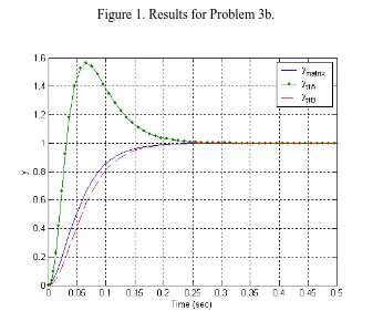
a) Implement (Simulink/Matlab) a state observer (not the transfer function) with state variable feedback for the one degree of freedom system on the web. Assume the state feedback gain is chosen so the closed loop poles are at p = [ -20 -30], the initial position and velocity of the true system are both zero, and the initial estimated position is 1 cm and the initial estimate velocity is -5 cm/s. You should be sure to include a prefilter. We are going to be examining the unit step response in this problem.

b) If the observer poles are also at p, you should get the response shown in Figure 1. c) Change the observer poles to 2*p, 4*p, and 8*p. Plot the results for each case. You should notice two things: (1) as the observer poles get farther away from the

estimates, particularly for the slopes, can be quick bad. This manifests itself as larger and larger control effort. Turn in all of these plots and Matlab/Simulink code for one case. d) Copy your observer/controller from part (a) to new files (Copy both the Matlab and Simulink files.). In addition to this state space based model, implement an

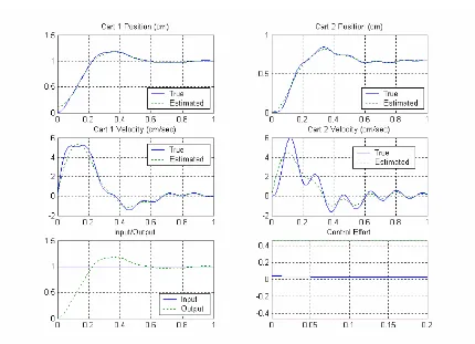
observer/controller transfer function as suggested on page 869 of the text (Program 12-8) for both types of configurations above. Assume for all systems that the closed loop state feedback poles are at p = [-30 -40] and the observer poles are at 3p. Assume all initial states are zero. Note that you do not need to write your model of the plant as a transfer function (you can leave it as a state space model), though the observer/controller transfer function should be written as a transfer function. Be sure to include the proper prefilter. You should get results like those displayed in Figure 2. Turn in your plot and

Matlab/Simulink code.

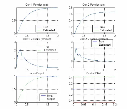
e) Implement (Simulink/Matlab) a state observer with state variable feedback configuration that forces the system to be a type one system for the one degree of freedom system with the state model on the web. Utilize an lqr controller, the last Q penalty value is a penalty on the new (augmented) state. Use the command k = lqr([0.1 0 1], 10). To determine the closed loop poles type p = eig(A-B*K). Set the observer poles equal to 2.5 times the state feedback poles (2.5*p). Set all initial states (observer, plant, and augmented state) to zero You should get results similar to those displayed in Figure 3. Turn in your plot and Matlab/Simulink code.

4) Two degree of freedom system.

a) Implement (Simulink/Matlab) a state observer (not the transfer function) with state variable feedback for the two degree of freedom system on the web. Assume the state feedback gain is chosen using the lqr method with K = lqr(A,B,diag([1 0.1 1 0.1],1e4)]. To determine the closed loop poles type p = eig(A-B*K).The initial position and velocity of both carts are both zero. The initial estimated position of the first cart is 0.1. All other initial estimates are zero. You should be sure to include a prefilter. We are going to be examining the unit step response in this problem.

b) If the observer poles are also at p, the position of the second cart is the only output available to the observer, and we are controlling the position of the first cart, you should get the response shown in Figure 4.

c) Change the observer poles to 2*p, 4*p, and 8*p. Plot the results for each case. You should notice two things: (1) as the observer poles get farther away from the

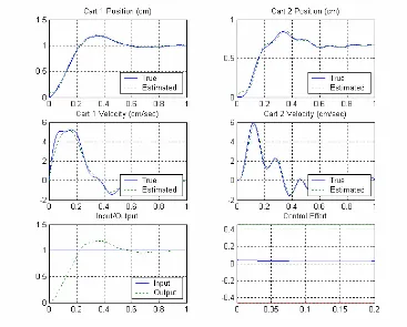
d) Repeat part (b), but assume the only output available to the observer is the position of the first cart and we want to control the position of the second cart. Turn in your plot. e) Repeat part (b), but utilize both the position of the first and second carts in the observer. You should get results similar to those in Figure 5. Turn in your plot. f) Copy your observer/controller from part (a) to new files (Matlab and Simulink). In addition to this state space based model, implement an observer/controller transfer function as suggested on page 869 of the text (Program 12-8) for both types of

configurations (A and B) above. (You should have three models all in one file.) Assume we are trying to control the position of the first cart and that the closed loop state

feedback poles are at p = [-20 -30 -25+5j -25-5j] and the observer poles are at p. Note that the only output available to the observer is the position of the first cart. Assume all initial states are zero. Note that you do not need to write your model of the plant as a transfer function (you can leave it as a state space model), though the observer/controller transfer function should be written as a transfer function. Be sure to include the proper prefilter. You should get results like those displayed in Figure 6. Turn in your plot and Matlab/Simulink code.

g) Change the location of the observer poles to 2*p, 3*p, 4*p, and 5*p. Which location gives the best result for the observer controller transfer function? Turn in your plots.

h) Repeart parts (f) and (g), but assume the only output available to the observer is the position of the second cart and we are trying to control the position of the second cart. Turn in your plots.

i) Implement (Simulink/Matlab) a state observer with state variable feedback configuration that forces the system to be a type one system for the two degree of freedom system with the state model on the web. Control the position of the first cart. Assume the positions of both carts are available for the observer. Utilize an lqr controller, the last Q penalty value is a penalty on the new (augmented) state. Use the command k = lqr([0.1 0 0.1 0 1], 1). To determine the closed loop poles type p = eig(A-B*K). Set the observer poles equal to 2.5 times the state feedback poles (2.5*p). Set all initial states (observer, plant, and augmented state) to zero.You should get results similar to those displayed in Figure 7. Turn in your plot and Matlab/Simulink code.

Figure 1. Results for Problem 3b.

Figure 3. Results for Problem 3e.

Figure 5. Results for 4e.