Possibilities of Using the Direct Runoff Model KINFIL for a Road Network Design

In the regions where agricultural and/or forestry production prevails, the road density is determined predominantly by economic criteria which reflect the requirements for optimal product transport. However, a different approach is adopted in regions where the production has a much lower priority. In such areas, limits should be placed on exces-sive construction of forest and field roads as too a dense road network would disturb the natural character of the landscape. Furthermore, the associ-ated drainage elements often create an unsuitable runoff system. Literature survey indicates that an optimal density of forest roads should be within the range of 7 to 14 m/ha (KLČ 2005).

In off-production areas, the ground slope, land use and soil water conditions should be the most important factors for a road network design when preparing land management projects. Depend-ing on these physiographic factors of individual sub-catchments formed by a road network, safe direct runoff from torrential rains is of the highest

required for agricultural or forestry road design projects. This requires rainfall-runoff analyses for different rain gauge stations located at altitudes ranging from 100 to 1200 m above the sea level (for the Czech conditions). Thus hydrological practitioners and design engineers can apply the described hydrological method in their road net-work design projects.

METHODS AND MATERIAL

The KINFIL model is based on the combination of infiltration theory with the transformation of direct runoff by a “kinematic wave”. The model uses the physiographic factor of a catchment as well as its hydraulic and soil parameters that can be derived either from field measurements or from map analyses. It can be implemented on ungauged catchments with no runoff data. The model is primarily intended for the design of dis-charge assessment for various catchment scenario

Possibilities of Using the Direct Runoff Model KINFIL

for a Road Network Design

PAVEL KOVÁŘ

_{, ŠÁRKA DVOŘÁKOVÁ}

_{and ELIŠKA KUBÁTOVÁ}

1

_{Department of Land Use and Improvement, Faculty of Forestry and Environment,}

and

_{Department of Mathematics, Technical Faculty, Czech University of Agriculture}

in Prague, Prague, Czech Republic

Abstract: The paper provides a practical implementation of the hydrological model KINFIL to be used for design-ing an optimal road density system in areas where agricultural or forestry production does not play an important role. In particular, such a road system project is based on the physiographic characteristics of land. Input data for a direct runoff analysis are computed in relation to the geometric parameters of upstream sub-catchments using the method of maximum daily precipitation reduction. Computed direct runoff discharges depend mainly on soil and vegetation conditions. Besides the soil type characteristics, the length and the angle of hill slopes to be drained by a road drainage system are major parameters determining the road density. These discharges are further assessed for road drain capacities designed according to the Czech Standard System (ČSN).

deforestation, urbanisation, etc. Its present ver-sion is based on the Green and Ampt infiltration theory, introducing the “ponding time” according to Morel-Seytoux (MOREL-SEYTOUX & VERDIN 1981).

The KINFIL model uses indirectly the Curve Number (CN) method (CHOW et al. 1988) but suppressing its weak physical background through the substitution of the common empirical CN approach by the physically based infiltration ap-proach. Therefore, the correspondence between CN values and saturated hydraulic conductivity

Ks and storage suction factor _Sf at field capacity was found earlier and these relationships were implemented in this paper (MOREL-SEYTOUX & VERDIN 1981; KOVÁŘ 1990). The regression analysis relationships as CN = f (K_s, S_f) and these pair values were performed for 62 stations in the Czech Republic, each for a duration of 30, 60, 90, 120, 180 and 300 min derived from daily (24 h) rainfalls with the return period of 1, 2, 5, 10, 20, 50 and 100 years with 7 major textural soil classes (Novak’s classification in KUTÍLEK 1978).

The second basic component of the KINFIL model is that representing direct runoff simula-tion. This process is based on a kinematic flow ap-proximation. Equation (1) expresses the kinematic wave describing an unsteady flow on a plane with different topographical characteristics:

(1)

where:

x – length (m)

y – depth (m)

t – time (s)

α_{, m – hydraulic parameters}

i_e(t) – effective rainfall intensity (m/s)

For the numerical solution, the explicit Lax-Wen-droff (L-W) finite difference scheme was imple-mented in the model (KOVÁŘ 1992). In principle, three simulation components, cascade of planes, converging or diverging segments and channel reaches can be used for the simulation of catch-ment topography. Practically, only planes were implemented in this project. The initial conditions of the L-W scheme were specified as y (x, 0) = 0 for all x. The upstream boundary depth was de-termined by the position of the plane in a cascade, when only one plane, then y (t, 0) = 0.

Design rainfalls

The tables of maximum one-day rainfalls in Czechoslovakia (ŠAMAJ et al. 1983) providing rain-fall depths were used for their reduction expressing the design depths and intensities for various dura-tion and probabilities according to the following formulae (HRÁDEK & KOVÁŘ 1994):

(2)

(3)

where:

t – duration of rain (min)

H_t,N – depth of rainfall with duration t and return period

N (mm)

i_t,N – intensity of rainfall with duration t and return period N (mm/min)

H_1d,N – maximum daily rainfall with return period N

(mm)

a, c – reduction coefficients

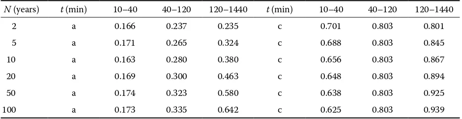
The design rainfalls for various duration t and different return periods N were determined as

Table 1. The reduction coefficient values for the design rainfalls

N (years) t (min) 10–40 40–120 120–1440 t (min) 10–40 40–120 120–1440

2 a 0.166 0.237 0.235 c 0.701 0.803 0.801

5 a 0.171 0.265 0.324 c 0.688 0.803 0.845

10 a 0.163 0.280 0.380 c 0.656 0.803 0.867

20 a 0.169 0.300 0.463 c 0.648 0.803 0.894

50 a 0.174 0.323 0.580 c 0.638 0.803 0.925

100 a 0.173 0.335 0.642 c 0.625 0.803 0.939

) (

1 _{i t}

t y my t y

e

m _�

� � �

�

� _� �

c N

d N

t H a t

H _{� � �} 1� ,

1 ,

c N

d N

t H a t

i _{� � �} �

mentioned above. As an example, the paper pro-vides the computation of the rainfall observatory station at Prachatice at an altitude of 642 m above the sea level. This station was selected as a repre-sentative example with high rainfalls.

The values of reduction coefficients a, c for the design rainfalls of various duration are given in Table 1.

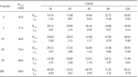
The values H_t,N in Table 2 represent maximum one-day rainfalls to be reduced to shorter design rainfalls of the duration 10 to 120 min for N return periods. This table is also graphically presented

as Figure 1 (rainfall depths) and Figure 2 (rainfall intensities).

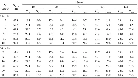
Table 3 provides the design effective rainfalls subtracting the infiltration and the retention com-ponents as the KINFIL model transforms direct runoff simulated by the kinematic wave from the effective design rainfall.

Infiltration and retention capacities in catch-ments are characterised by the Curve Number CN. For a selected sub-catchment hydrological soil groups C and D were considered where average CN values are CN = 80 and CN = 88, resp. Table 2. Design rainfall depths and intensities for the Prachatice station

N (years) H1d,N (mm)

t (min)

10 20 30 60 120

2 42.8 Ht,N 14.14 17.40 19.64 22.72 26.05

i_t,N 1.41 0.87 0.65 0.38 0.22

5 57.4 Ht,N 20.13 24.99 28.36 34.08 39.06

i_t,N 2.01 1.25 0.95 0.57 0.33

10 66.8 Ht,N 24.04 30.52 35.08 41.90 48.03

i_t,N 2.40 1.53 1.17 0.70 0.40

20 76.6 Ht,N 29.11 37.16 42.86 51.48 59.01

i_t,N 2.91 1.86 1.43 0.86 0.49

50 88.6 Ht,N 35.48 45.60 52.81 64.11 73.49

i_t,N 3.55 2.28 1.76 1.07 0.61

100 98.0 Ht,N 40.20 52.14 60.70 73.55 84.31

i_t,N 4.02 2.61 2.02 1.23 0.70

0 20 40 60 80 100

0 10 20 30 40 50 60 70 80 90 100 110 120

Rainfall

depth

Ht,N

(m

m

)

N = 2 N = 5 N = 10

N = 20 N = 50 N = 100

Figure 1. Design rainfall depths for duration 10–120 min and for return periods N years (Pracha-N = 2

N = 20

N = 5

N = 50

N = 10

The depths of effective rainfalls are computed from equations (4) and (5).

(4)

A = 25 400.0 – 254 (5)

CN where:

H_et,N – depth of effective design rainfall with duration and return period N (mm)

A – potential retention (mm)

RESULTS

The simplest way to drain water out of a road network system is to construct open ditches along the road as a lateral drain element catching runoff from upstream slopes.

These ditches are usually made in either trian-gular or trapezoidal cross-sections. The latter is better as it is hydraulically more effective concern-ing the larger cross-section profile at the same water depth in a ditch. Its design concerning forest 0

1 2 3 4 5

0 10 20 30 40 50 60 70 80 90 100 110 120

Rainfall duration (min)

Rainfall intensitie (mm/min)

N = 2 N = 5 N = 10 N = 20 N = 50 N = 100

Figure 2. Design rainfall inten-sities for duration 10–120 min and for return periods N years (Prachatice)

Table 3. Depth of effective design rainfalls (Station Prachatice 642 m above the sea level)

N

(years) (mm)H1d,N

t (min)

10 20 30 60 120

H_t,N H_et,N H_t,N H_et,N H_t,N H_et,N H_t,N H_et,N H_t,N H_et,N

CN = 80

2 42.8 14.1 0.0 17.4 0.3 19.6 0.7 22.7 1.4 26.1 2.3

5 57.4 20.1 0.8 25.0 2.0 28.3 3.1 34.1 5.4 40.0 8.2

10 66.8 24.0 1.7 31.0 4.1 35.1 5.8 42.0 9.3 48.0 12.6

20 76.6 29.1 3.4 37.2 6.8 42.9 9.7 51.5 14.7 59.0 19.5

50 88.6 35.5 6.0 45.6 11.2 52.8 15.5 64.1 23.0 73.5 29.7 100 98.0 40.2 8.3 52.1 15.1 60.7 20.7 73.6 29.8 84.3 37.9 CN = 88

2 35.6 14.1 1.2 17.4 2.4 19.6 3.4 22.7 4.9 26.1 6.8

5 48.4 20.1 3.6 25.0 6.2 28.3 8.2 34.1 11.9 40.0 16.2

10 56.6 24.0 5.6 31.0 9.9 35.1 12.6 42.0 17.6 48.0 22.3

20 65.2 29.1 8.7 37.2 14.1 42.9 18.3 51.5 25.1 59.0 31.3 50 75.7 35.5 12.9 45.6 20.4 52.8 26.1 64.1 35.6 73.5 43.8 100 83.9 40.2 16.3 52.1 25.6 60.7 32.7 73.6 43.9 84.3 53.4

A H

A H

H

N t

N t N

et _{� �}

� � �

8 . 0

) 2 . 0 (

,

2 ,

,

N = 2

N = 20

N = 5

N = 50

N = 10

roads is given in the Czech Standard: ČSN 73 6108 including the basic parameters as follows: bottom width b = 0.40 m

depth of ditch H = 0.50 m

bank slopes l:1

Its minimum longitudinal slope J is proposed to 0.5% in the ČSN. As an optimum longitudinal slope

J = 1% (lowlands) and maximum J = 3% (highlands) were considered. The ditch discharge capacity was calculated from the continuity equation:

Q = Sv (m3_{/s) (6)}

where:

S – cross-section area (m2₎ v – flow velocity (m/s)

The trapezoidal cross-section area S with the parameters above was calculated.

The flow velocity in a ditch is computed by the Chézy equation:

v = C√RJ (m/s) (7)

where:

C – Chézy coefficient (m1/2_/s) R – hydraulic radius (m)

J – longitudinal slope

C = 1 R1/4 _(m1/2_{/s) (8)}

n where:

n – Manning roughness coefficient, for a grassland ditch n = 0.025

Then the flow velocity is computed for all three longitudinal bottom slopes of ditch.

v_min = 31.75 √0.25 × 0.015 = 1.12 (m/s)

v_opt = 31.75 √0.25 × 0.01 = 1.59 (m/s)

v_max = 31.75 √0.25 × 0.03 = 2.75 (m/s) The adequate discharges are:

Q_min = 0.45 × 1.12 = 0.51 (m3_/s)

Q_opt = 0.45 × 1.59 = 0.72 (m3_/s)

Q_max = 0.45 × 2.75 = 1.24 (m3_/s)

Concerning the agricultural road network pro-posal and their drainage systems, they are based on the Czech standard ČSN 73 6109 and it is simi-larly so for the forest road system. Therefore, this system is not considered in this paper.

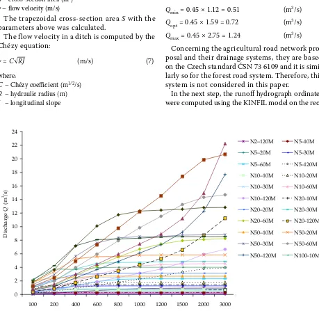
In the next step, the runoff hydrograph ordinates were computed using the KINFIL model on the

rec-0 2 4 6 8 10 12 14 16 18 20 22 24

100 200 400 600 800 1000 1200 1500 2000 3000 Slope lenght L (m)

D

is

ch

ar

ge

Q

(m

3 /s

)

N2–10M N2–20M N2–30M N2–60M N2–120M N5–10M N5–20M N5–30M N5–60M N5–120M N10–10M N10–20M N10–30M N10–60M N10–120M N20–10M N20–20M N20–30M N20–60M N20–120M N50–10M N50–20M N50–30M N50–60M N50–120M N100–10M N100–20M

N2–10M N2–20M N2–30M N2–60M N2–120M N5–10M N5–20M N5–30M N5–60M N5–120M N10–10M N10–20M N10–30M N10–60M N10–120M N20–10M N20–20M N20–30M N20–60M N20–120M N50–10M N50–20M N50–30M N50–60M N50–120M N100–10M

tangular plane with various slopes simulating field conditions. The plane width was determined constant, which equals the theoretical length of the ditch,

b = 1000 m. This length can be easily determined as unity length for better calculation for any specific length on design request. In practice, the ditch length

is usually shorter. The slopes were considered as 1%, 3%, 5%, 7%, 10%, 12% and 15%. For each of them their length was considered as 100, 200, 400, 600, 800, 1000, 1200, 1500, 2000 and 3000 m. Due to the wide range of computed results, only some illustra-tive examples are published in the paper.

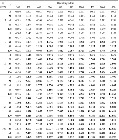
Table 4. Design discharges Q (m3_{/s) in the standard road ditch for the characteristics of design effective rainfalls and} for given ditch length (1000 m), soil group (D) and hill slope (15%) – Prachatice Station; CN = 88

N (year) D

Ditch length (m)

100 200 400 600 800 1000 1200 1500 2000 3000

2

10 0.050 0.051 0.051 0.051 0.051 0.051 0.051 0.051 0.051 0.051 20 0.150 0.159 0.164 0.164 0.164 0.164 0.164 0.164 0.164 0.164 30 0.183 0.276 0.290 0.291 0.291 0.291 0.291 0.291 0.291 0.291 60 0.137 0.274 0.488 0.531 0.540 0.542 0.542 0.542 0.542 0.542 120 0.095 0.190 0.382 0.574 0.752 0.862 0.908 0.929 0.939 0.940

5

10 0.295 0.312 0.322 0.322 0.322 0.322 0.322 0.322 0.322 0.322 20 0.477 0.742 0.782 0.798 0.798 0.798 0.798 0.798 0.798 0.798 30 0.425 0.873 1.219 1.246 1.268 1.270 1.270 1.270 1.270 1.270

60 0.330 0.661 1.321 1.905 2.211 2.303 2.325 2.325 2.325 2.325

120 0.225 0.450 0.903 1.356 1.812 2.267 2.721 3.298 3.779 3.943

10

10 0.633 0.618 0.673 0.673 0.673 0.673 0.673 0.673 0.673 0.673 20 0.823 1.423 1.669 1.726 1.742 1.744 1.744 1.744 1.744 1.744

30 0.701 1.380 2.339 2.523 2.558 2.600 2.607 2.608 2.608 2.608

60 0.481 0.978 1.956 2.923 3.732 4.198 4.389 4.468 4.535 4.549

120 0.310 0.621 1.241 1.867 2.493 3.120 3.748 4.685 5.906 6.652

20

10 1.204 1.290 1.386 1.405 1.405 1.405 1.405 1.405 1.405 1.405

20 1.175 2.171 2.985 3.017 3.127 3.145 3.147 3.147 3.148 3.148

30 1.018 2.021 3.777 4.576 4.712 4.750 4.836 4.861 4.865 4.865

60 0.697 1.395 2.790 4.186 5.545 6.684 7.432 7.927 8.098 8.228

120 0.435 0.871 1.742 2.617 3.494 4.373 5.252 6.574 8.736 11.250

50

10 1.960 2.488 2.490 2.702 2.712 2.713 2.713 2.713 2.713 2.713

20 1.701 3.371 5.263 5.576 5.594 5.786 5.823 5.831 5.832 5.832

30 1.451 2.903 5.628 7.594 8.357 8.521 8.551 8.743 8.797 8.801

60 0.989 1.979 3.957 5.937 7.917 9.840 11.528 13.260 14.320 14.686

120 0.609 1.218 2.436 3.656 4.880 6.108 7.335 9.180 12.251 17.685

100

10 2.253 3.758 3.681 3.948 4.005 4.009 4.010 4.010 4.010 4.010

20 2.116 4.251 7.185 8.087 8.163 8.305 8.469 8.515 8.521 8.522

30 1.819 3.637 7.143 10.077 11.736 12.294 12.429 12.556 12.798 12.825

60 1.221 2.443 4.885 7.328 9.774 12.208 14.530 17.397 19.846 20.657

Thus the design discharges in lateral road ditches in the territory with the altitude of 600 to 700 m above the sea level (e.g. Prachatice) and with soil group D were computed. These results were in-cluded in Table 4 and plotted in Figure 3. It is evident that the tabled results in bold overtop the discharge capacity of standard ditches and consequently do not guarantee their safe “in-bank” outflow (within the Czech Standard, ČSN).

DISCUSSION

The applied KINFIL model version was adapted for this unsteady flow over the rectangular plane on purpose. Thus due to a large range of computations and due to the requested solution flexibility the simplest model configuration was implemented. The kinematic wave principle considering un-steady but uniform flow is hydraulically correct and seems to be adequate to natural situation when no back-flow is expected. This model also offers a more sophisticated solution when the topographi-cal prototype can be better simulated using not only the “rectangular plane model” but also its combination with segments either convergent or divergent (KOVÁŘ et al. 2002). However, such a specific solution would exceed a “general solution” introducing certain specific topography hardly usable for the high majority of events. Instead of the very flexible use of CN values, the model offers also other hydraulic soil parameter implementa-tion (e.g. K_s , S_f). Its numerical scheme is stable and in the case of failure it enables to shorten the computational time step during computation on a PC (from the keyboard). It is assumed that consulting engineers, as users of this method, can quickly incorporate the solution of an unsteady water flow through the road ditch system. This physically based method can upgrade the scientific level of a rural road system design.

CONCLUSIONS

This case study represents a hydrological situa-tion which is consistent with the posisitua-tion of Pra-chatice station (600 to 700 m above the sea level), hydrological soil group D and the plane slope 15%. Results printed in bold in Table 4 show discharges exceeding the ditch capacities, i.e. higher than maximum discharge capacities of standard ditches (ČSN). It is obvious that concerning the forest and

only rainfalls with return period less than N = 2 years (at most N = 5 years) are rational, other-wise these systems would be over-dimensioned. Therefore, the adequate “bold-parts” of the tables have to be avoided.

In general, it can also be concluded that this method brings the results comparable with the results of a broadly used kinematic wave method (OVERTON & MEADOWS 1976) from the end of the 1970s to the present time. However, this method has not yet been used in practical project design and therefore we point out that its application should always be confronted in the context of other requirements of a common transport sys-tem. It should also be emphasized that this paper only concerns the rainfall-runoff problems when a road design is conceived.

References

CHOW V.T., MAIDMENT D.R., MAYS L.W. (1988): Applied Hydrology. McGraw Hill, New York.

ČSN 73 6108: Lesní dopravní síť. Český normalizační institut, Praha.

ČSN 73 6109: Projektování polních cest. Český norma-lizační institut, Praha.

HRÁDEK F., KOVÁŘ P. (1994): Výpočet náhradních intenzit přívalových dešťů. Vodní hospodářství, 11: 49–53. KLČ P. (2005): Research on principles of making access

to mountain forests by forest road network. Journal of Forest Science, 51: 115–126.

KOVÁŘ P. (1990): Application of Adapted Curve Number Model on the Sputka Catchment. Hydrology of Moun-tainous Areas. IAHS Publication No. 190. IAHS Press, Wallingford, 391–401.

KOVÁŘ P. (1992): Possibilities to determine design dis-charges on small catchments by the KINFIL model. (in Czech with English abstract) Journal of Hydrology and Hydromechanics/Vodohospodársky časopis, 40: 197–220.

KOVÁŘ P., CUDLÍN P., HEŘMAN M., ZEMEK F., KORY-TÁŘ M. (2002): Analysis of flood events on small river catchments using the KINFIL model. Journal of Hyd-rology and Hydromechanics, 50: 157–171.

KUTÍLEK M. (1978): Vodohospodářská pedologie. SNTL/ ALFA, Praha/Bratislava.

Corresponding author:

Prof. Ing. PAVEL KOVÁŘ, DrSc. Česká zemědělská univerzita v Praze, Fakulta lesnická a environmentální, katedra biotechnických úprav krajiny, Kamýcká 129, 165 21 Praha 6-Suchdol, Česká republika

tel.: +420 224 382 148, fax: +420 234 381 848, e-mail: kovar@fle.czu.cz ŠAMAJ F., BRÁZDIL R., VALOVIČ J. (1983): Denné úhrny

zrážok s mimoriadnou vydatnosťou v ČSSR v období 1901–1980. In: Sborník prác SHMÚ. ALFA, Bratislava, 19–112.

Technická doporučení pro lesní dopravní síť. Ministerstvo zemědělství ČR, odvětví lesního hospodářství, Praha.