Novel Numerical Simulation of the Stereological Bias of Binary Particles

Stereological correction, which corrects an overestimation of the degree of liberation of minerals in a two-dimensional measurement, has not been adequately established, despite its importance in the evaluation of not only the crushed product but also the efficiency of comminution and sorting in the mining process. A unique numerical method was conducted using Discrete Element Method in order to investigate the relationship between the two-dimensional information obtained by cross-sectional measurement and three-dimensional practical information. First, spherical particles of a certain-sized dispersion were packed in a sampling cell. Following this, phases with a lognormally distributed volume fraction, which was designated by a medianMDand standard deviationSD, were placed between the particles. Finally, the serial sectional information was analyzed in the height direction, and the following fundamental results were obtained: 1) the area fraction of the cross-sectional circles distributed around the practical volumetric fraction and 2) the degree of liberation was overestimated by the two-dimensional cross-sectional measurement. A series of parametric studies was then conducted on the phases using variousMD and SDvalues, and a correlation between the two-dimensionally measured and three-dimensional actual parameters was obtained. In using this correlation, the volumetric distribution of the phase, together with its degree of liberation (which is usually difficult to measure directly), was estimated with parameters obtained by cross-sectional measurement, such as optical microscopy, QEM*SEM, and MLA. This was based on the assumption that all the particles include a single spherical phase with a lognormally distributed volume. [doi:10.2320/matertrans.M-M2016801]

(Received October 7, 2015; Accepted December 16, 2015; Published February 25, 2016) Keywords: mineral liberation, stereological bias, discrete element method

1. Introduction

It is essential to liberate valuable phases in mineral processing because the degree of liberation determines the ultimate limit of the separation. At present, however, a liberation evaluation method has not been fully established. It is difficult to evaluate not only the crushed product but also the efficiencies of the comminution and sorting methods without an appropriate evaluation of the liberation. The establishment of a liberation evaluation technique represents a technical breakthrough in thefields of mining and recycling engineering.

X-ray CT analysis and the subsequent image processing directly obtain the three-dimensional internal structure of minerals and the degree of liberation.1) However, from a practical perspective, there are challenges in the segregation of minerals with similar specific gravities and in the scanning speed. Optical microscopes have been commonly used for two-dimensional measurement of a sectional area or linear intercepts on the polished section of mineral particles.2)

However, this method is time-consuming and includes uncertainty resulting from the manual measurement.3)

Recently, automated mineral analyzing systems such as mineral liberation analyzer (MLA)3)_{and quantitative electron}

microscopy­scanning electron microscopy (QEM*SEM),4)

which are a combination of back-scattered electron and X-ray analyses, have become popular. It is well known, however, that these two-dimensional measurement methods overestimate the degree of liberation. This is called“ stereo-logical bias”because a randomly derived cross-section may not intersect all phases of the particles.5,6)It has been reported that stereological bias is an important consideration when most particles are composite and their textures are simple.4,6,7)

Various attempts have been made to overcome stereo-logical bias. In general, as far as well-examined samples are

concerned, three-dimensional liberation data are successfully estimated by two-dimensional measurements using several methods: the actual liberation percentage is simply calculated by dividing the two-dimensional apparent liberation percent-age by an empirical correction factor;8,9) _{the true liberation}

distribution is estimated from areal or line measurement using a transformation kernel.5,10)_{In order to expand the versatility}

of the above-mentioned research outcome, further research progress from a general perspective is required.

Discrete Element Method (DEM)11) _{is a powerful tool}

for numerically simulating randomly packed particles and rapidly investigating their internal structure free from any experimental errors. It is useful in obtaining a basic idea of a complicated problem, such as liberation analysis, which is influenced by many factors for which exhaustive experimen-tal characterization is difficult.

We conducted a series of unique numerical simulations consisting of three parts: particle packing by DEM, modeling of inter-particle composition, and serial cross-sectional analysis in the height direction. By comparing the two-dimensional information obtained from the serial cross-sectional analysis and true three-dimensional information, a correlation was found, which enables us to predict the volumetric distribution of a phase included in the particles by a two-dimensional measurement only.

2. Methodology

2.1 Particle packing simulation by DEM

adequately decayed. It was confirmed by preliminary simulation that the effects of the packing state (e.g., packing density) on the parameters obtained by cross-sectional measurement were negligible.

2.2 Modeling of inter-particle composition

As afirst step, we considered particles of relatively simple texture, whose stereological bias is great.4,6,7)Figure 3 shows a schematic image of the particle simulated in this study. The particle consists of two phases: phase A, which is a concentric sphere that does not exceed the particle size, and phase B, which is the remainder of particle. As afirst step in evaluating this numerical method, a relatively simple particle was modeled. In addition, it has been reported that binary particles consisting of shells of one phase surrounded by another phase are produced by the breakage of ores containing one hard phase, such as pyrite, and soft phases, such as chalcocite, bornite, or galena.8)_{The stereological bias}

of these particles should be predicted because of its negative influence onflotation efficiency.

The overall volume fraction of phase A of all the particles,

FV, and that of each particle,fV, were defined as follows:

FV¼_ð ðTotal volume of phase AÞ

Total volume of the particlesÞ ð1Þ

fV¼

ðVolume of phase A in a prticleÞ

ðVolume of a particleÞ ; ð2Þ

In the present study,fVwas arbitrary given in the range from

0 to 1, andFVwas calculated as a result offV. For example,

whenfVis given as afixed value, e.g.,fV=0.1,FVbecomes

equivalent to fV i.e., FV=fV=0.1. However, when fV is

given as distributed values, as explained in the later section,

FVis calculated as a result offVof all particles.

2.3 Serial cross-sectional analysis of the particle assem-bly

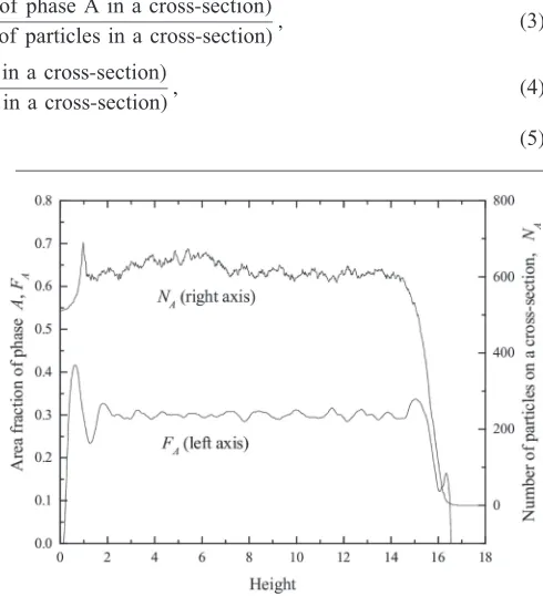
Serial cross-sectional information was geometrically cal-culated in the height direction, as shown in Fig. 2(a), as a schematic image. Figure 2(b) shows the cross-sectional data, and Fig. 2(c) shows an enlarged image of Fig. 2(b) as examples in the case ofFV=0.1. Phases A and B are

color-coded in the figures. Apparently liberated particles were observed despiteFV=0.1: namely every particle has a phase

A with a volumetric fraction of 0.1. Some parameters used in the two-dimensional analysis such as the area fraction of phase A,FA, the degree of presence of phase A,DA, and the

degree of apparent liberation of phase B,DLB, were defined

as follows:

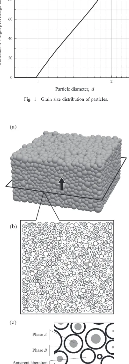
Fig. 1 Grain size distribution of particles.

Fig. 2 Schematic images of the simulation: (a) the packed particles with size ranging from 1.0 to 2.0 [Fig. 1], where the serial cross-sectional data is acquired in the height direction; (b) an example of a cross-sectional image; (c) an enlargement of the cross-sectional image (b), where the phases A and B are color-coded, and apparently liberated particles are observed.

measurement and range from 0 to 1. Note that for

convenience in the measurement, DA and DLB were

calculated from the ratio of the numbers, not the areas. In addition, FA,DA, and DLB are parameters that can be

obtained by two-dimensional measurement, such as optical microscopy, QEM*SEM, and MLA.

3. Numerical Analysis

3.1 Determination of the simulation parameters 3.1.1 Cross-sectional measurement range

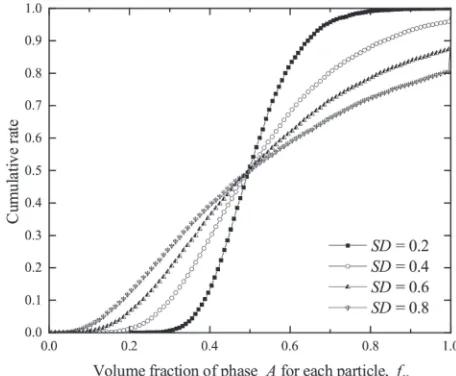
Figure 4 plots the area fraction of phase A, FA, and the

number of particles in a cross-sectionNAagainst the height of

the cross-section Hof the sample whoseFVis 0.3. Both FA

andNAshow a peak aroundH=1.0, become stable whenH

is in the range from 1.0 to 14.0, and suddenly decrease when

His over 14.0. The peak values ofFAandNAaroundH=1.0

are thought to be caused by particles on the bottom plate, which were relatively regular in their arrangement. The sharp decreases ofFAandNAwhenHis more than 14 are caused by

the top-edge effects of the sample.

In this study, in consideration of the two above-mentioned effects, cross-sectional analysis was conducted in the range of

Hfrom 2 to 14.

3.1.2 The interval and the number of the cross-sections

A series of preliminary simulations was conducted to clarify the parameters of the cross-sections. It was confirmed that stable cross-sectional data is available in cases where the interval of the cross-section is set to be less than 1/5 of the smallest particle diameter. In this study, the cross-section interval was set to be 1/20 of the smallest particle diameter.

Similarly, it was found that stable average values are obtained in the cases where the number of analyzed cross-sections is over 150, whereas the dispersion decreases as the number of cross-sections increases. In this study, the number of analyzed cross-sections was set at 600.

3.1.3 Cross-sectional area of the samples

Figure 5 shows the cumulative curve ofFAfor the sample

whose FVis 0.3 packed in various widths of the sampling

cell,W=10, 30, 50, and 70. The depth of the sampling cell took the same value asW; therefore, the samples had square-shaped cross-sections. The figure shows a wide distribution when W=10 and narrower and similar distributions when

W²30, aroundFA=0.3 in each case. Considering that the

integral ofFAisFV, statistically reliable data can be obtained

in cases whereW²30. We appliedW=30 in this study. The present study was conducted on the particles with dimensionless size, but corresponding dimensional size in mm was computed. Table 1 shows the corresponding particle size calculated from the ratio of the cross-sectional areas of the largest particles, smallest particles, and sampling cell, on

Fig. 4 The area fraction of phase A,FA, and the number of particles in a

cross-section,NA, are plotted against the height of the cross-section,H.

Volume fraction of phase A,FV, is 0.3, and particle diameter ranging from

1 to 2.

Fig. 5 Cumulative curves of the area fraction of the phase A,FA, with

various sample sizes.

Table 1 Corresponding particle sizes.

W Corresponding maximum

diameter (mm)

Corresponding minimum diameter (mm)

10 5.32 2.66

30 1.77 0.89

50 1.06 0.53

the assumption that the sampling cell has an equivalent sectional area to the 30-mm-diameter mold.3)

3.2 Simulation

We considered two types of particles: those having afixed volume fractionfVof phase A (i.e., the“fixed fVcase”) and

those having a lognormally distributedfV(i.e., the“dispersed

fVcase”). Figure 6 describes the basic idea of the dispersed

fV case. Figure 6(a) conceptually depicts the original,

pre-crushed, state of phases A and B, where the dispersed phase A is embedded in the continuous part of phase B. The volume of phase A has a lognormal distribution. In the situation where the material was crushed to be the size of the mesh, it was found that phase A was smaller than the mesh [Fig. 6(a)(i)], and thefVvalue of the particle corresponded to

the size of phase A. Meanwhile, if the size of phase A was larger than that of the mesh [Fig. 6(a)(ii)], the liberated phase A,fVbecame one becausefVcannot exceed one, according to

the definition of eq. (2). Therefore, as shown in Fig. 6(b), the distribution of fV for the dispersed fV case was set with

respect to the lognormal distribution, andfVwas modified to

one for the range where the distribution exceeded one [see the right tail of the distribution in Fig. 6(b)].

FVwas equivalent to the designatedfVvalue in thefixedfV

case. In the dispersed fV case, on the other hand, the fV

distribution was determined by the designated values of the median MD and the logarithmic standard deviation of fV

(SD), respectively. Specifically, in the case MD=0.5 and

SD=0.2,fVis distributed around 0.5, and 68%of particles

have anfVranging from 0.3 to 0.7.

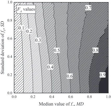
Figure 7 shows the cumulative fV curves of the sample

whose MDis 0.5 and whoseSDsare 0.2, 0.4, 0.5, and 0.8. Table 2 presents the simulation cases.

Figure 8 depicts the cross-sectional images of the samples: (a) withfixedfV, whoseFVwas 0.4 and (b) with dispersedfV,

whoseFV=0.4 (MD=0.3,SD=0.8), respectively,

togeth-er with the partially enlarged images. A largtogeth-er numbtogeth-er of apparently liberated particles are observed in the dispersedfV

case [Fig. 8(b)] due to the fVdispersion compared with the

fixed fVcase [Fig. 8(a)].

4. Results and Discussion

4.1 Simulation results

Starting from the basic case, the fixed fV cases were

investigated. To investigate the effects of the volume fraction of phase A,FVfor the degree of presence of phase A,DA, and

the degree of apparent liberation of phase B, DLB, the

samples with fixed fV, whose FV=0.1, 0.3, and 0.5, were

investigated.

Figure 9 shows the cumulative curves of DA and DLB

for the three cases. DA increases drastically, whereas DLB

decreases with increasingFV. The relationships betweenFV,

DA, and DLB are discussed later from the perspective of

geometry. It should be emphasized here that the two-dimensional measurement ofDAandDLBwere quite different

from the three-dimensional practical conditions, where all of the particles included phase A. Hence, the ideal values ofDA

and DLB were one and zero, respectively, and the

stereo-logical bias was great in these cases.

Subsequently, in order to inquire on the association between two-dimensional measured information and three-dimensional practical information a series of parametric

studies on MD and SD was conducted. These studies

involved 10,201 cases with combinations of 101 patterns of

MDand SDvarying from 0.0 to 1.0 in every 0.01.

Figure 10 shows the isogram of the apparent liberation of phase B, DLB, with respect to MD and SD. DLB is caused

entirely by the stereological bias because there is no truly liberated phase B in this simulation. DLB increases with

decreasing MD: it reaches about 20% when MDis 0.5 and about 40% whenMDis 0.2.

In order to assess the correlation betweenMDandSD, and the degree of liberation of phase A in 3D,D3D

A, is defined as

follows:

D3D A ¼

Number of particles liberated with phase A Number of particles ð6Þ Fig. 6 Conceptual images offVdistribution in the dispersedfVcase: (a) the

material, where phase A with lognormal distribution was embedded in phase B, was crushed to be the size of the mesh, and a particle was created; (b) the lognormal distribution offVin the dispersedfVcase.

Fig. 7 Cumulative rate offVfor the sample whoseMDis 0.5 with various

SDvalues.

Table 2 Simulation cases.

Fixedfv FV=0.1­0.9 in every 0.1

Dispersedfv

MD=0.0­1.0 in every 0.01

Figure 11 shows the isogram ofD3D

Awith respect toMDand

SD. D3D

A increases with both increasing MD and SD. In

this simulation, contrary to the phase B case, there is no stereological bias for phase A because phase A exists in the condition either being enveloped by phase B or by being liberated. As shown in Fig. 11, D3D

A is determined by its

volumetric distribution parameters, MD and SD. From this point forward, the relationship between the three-dimensional parameters of the volumetric distribution of phase A, MD, and SD, and the two-dimensional parameters in order to predict the three-dimensional information about phase A by two-dimensional measurement.

Figure 12 shows the isogram ofFA[eq. (3)] with respect

to MD and SD. FA has a positive correlation with MD,

whereas it has little correlation with SD.

Here, we need another parameter that is two-dimensionally measureable and is expected to have a correlation with SD, the standard deviation of the sectional area of phase A,·A.·A

is defined as follows:

·A¼_n1 Xn

1

Standard deviation of cross-sectional area of phase A on a cross-section

:

ð7Þ

Figure 13, which is the isogram of·Awith respect toMD

and SD, shows that·Ahas a positive correlation with SD.

4.2 Prediction of the phase A distribution in 3D

Figure 14, which is formed by the union of Fig. 12 and Fig. 13, plots all the simulation results with respect to the two-dimensional parametersFAand·A. Their parameters for

the three-dimensional distributions of phase A,MD, and SD

are shown by the color code and iso-line, respectively. The bottom curves show the cases whereSDis zero, namely the mono-sized particle cases. In these cases,·Ais caused only

by the randomness of the intersected particle positions;

Fig. 9 Cumulative curves of the degree of presence of phase A,DA, and the degree of liberation of phase B,DLB, with various volume fractions of phase A,FV.

0.60 0.50

0.40

0.30

0.20

0.10

0.0 0.2 0.4 0.6 0.8 1.0

0.0 0.2 0.4 0.6 0.8 1.0

D_LB values

Sta

ndard de

via

tion of

fV

,

SD

Median value of f_V,MD

Fig. 10 Isogram ofDLBvalues of the dispersedfVsamples withMDand SDranging from 0.0 to 1.0 in every 0.01.

Fig. 8 Cross-sectional images and close-up images of the samples together with their partially enlarged images (a) withfixedfV, whoseFVis 0.4, and

therefore, it is the lower limit in this simulation.·Aincreases

with increasing SD, because it is determined by the randomness of the particle sizes in addition to the random-ness of the intersected positions of the particles. The three-dimensional volumetric distribution of phase A can be predicted by two-dimensional measurement using Fig. 14. In addition, the degree of liberation is predicted by the intercept of the fVdistribution when fVis one, as shown in Fig. 6(b).

This model is based on the assumption that one spherical phase is located within the spherical particle. In order to demonstrate the applicability of the proposed numerical method to the stereological bias analysis, a relatively simple particle was modeled in this simulation. The model is considered to be applicable to binary particles consisting of shells of one hard phase, such as pyrite, surrounded by another soft phase, such as chalcocite, bornite, or galena.8)_In

addition, much realistic case of particles with random texture

will be reported in a later paper. An extended analysis of stereological bias for particles with a more realistic texture will be conducted based on the fundamental idea of the numerical method presented in this paper.

5. Conclusion

A series of numerical simulations was conducted to investigate the relationship between the two-dimensional information obtained by cross-sectional measurement and the three-dimensional practical information by the following steps:

(1) Spherical particles with a certain particle size dispersion were packed using Discrete Element Method.

(2) Phases with a lognormally distributed volume fraction, with a median MD and standard deviation SD, were placed inside the particles.

(3) Serial cross-sectional information was analyzed in the height direction.

0.9 0.8 0.7

0.6 0.5

0.4 0.3 0.2 0.1

0.0 0.2 0.4 0.6 0.8 1.0

0.0 0.2 0.4 0.6 0.8 1.0

Standard deviation of

fV

,

SD

Median value of f_V,MD F_A values

Fig. 12 Isogram ofFAvalues of the dispersedfVsamples withMDandSD

ranging from 0.0 to 1.0 in every 0.01.

Fig. 13 Isogram of·Avalues of the dispersedfVsamples withMDandSD

ranging from 0.0 to 1.0 in every 0.01.

Fig. 14 Relationship of three-dimensional parameters,MD and SD, and two-dimensional parameters,FAand·A, of all the dispersedfVcases.

A series of parametric studies was then conducted on the 10,201 patterns of phases with various MD and SD values, and a correlation between the two-dimensional measured and three-dimensional actual parameters was obtained. In the use of the correlation, the volumetric distribution of the phase, together with its degree of liberation (which is usually difficult to measure directly), was estimated by parameters that could be obtained by cross-sectional measurement. The correlation was developed on the basis of the assumption that all the spherical particles include a single spherical phase with a lognormally distributed volume.

5) J. D. Miller and C. L. Lin:Int. J. Miner. Process.22(1988) 41­58. 6) D. Lätti and B. J. I. Adair:Miner. Eng.14(2001) 1579­1587. 7) S. Spencer and D. Sutherland:Image Anal. Stereol.19(2000) 175­182. 8) A. M. Gaudin:Principles of Mineral Dressing, (McGraw-Hill Inc. US,

1939).

9) W. B. Petruk: Trans. Inst. Min. Metall. Sect. C87(1978) C272­C277. 10) R. P. King and C. L. Schneider:Powder Technol.98(1998) 21­37. 11) P. A. Cundall and O. D. L. Strack:Geotechnique29(1979) 47­65. 12) D. Weatherley: ESyS-Particle: HPC Discrete Element Modelling