On the Periodicity of 〈001〉 Symmetrical Tilt Grain Boundaries

On the Periodicity of

©

001

ª

Symmetrical Tilt Grain Boundaries

Kazutoshi Inoue

, Mitsuhiro Saito

, Zhongchang Wang

,

Motoko Kotani

and Yuichi Ikuhara

1_{WPI Research Center, Advanced Institute for Materials Research, Tohoku University, Sendai 980-8577, Japan} 2_{Institute of Engineering Innovation, School of Engineering, The University of Tokyo, Tokyo 113-8656, Japan}

We report an application of the O-lattice theory to systematically analyse the structures of symmetrical tilt grain boundaries with the rotation axis of©001ªand demonstrate a theoretical interpretation of the experimentally observed structures of a near­5 grain boundary in MgO in terms of the structural-units model and the periodicity of the O-points on the boundary. We further derive generalised decomposition formulae for the symmetrical tilt grain boundaries which are closely related to the distribution of irreducible rational numbers.

[doi:10.2320/matertrans.M2014394]

(Received November 7, 2014; Accepted December 16, 2014; Published February 6, 2015)

Keywords: atomic structure, crystal structure, dislocations, symmetrical tilt grain boundary, structural unit, O-lattice

1. Introduction

Grain boundaries with a large index rarely exist in nature, and can be decomposed into the ones with a smaller index due to relaxation. Over two decades ago, both symmetrical and asymmetrical tilt grain boundaries were intensively studied1­16) and a general consensus was that actual configurations of grain boundaries could be realised by arranging smaller structural units. Since then, numerous experiments and calculations on the grain boundary geo-metries have been conducted and the study of interfaces in crystalline materials was summarised by A. P. Sutton and R. W. Balluffi.17)_{R. C. Pond and his collaborators provided a}

general theoretical framework in regard to the symmetry of space groups and point groups on the dichromatic pattern and complex of two adjacent lattices18,19)_{that was closely related}

to the periodic appearance of structural units as energetically stable configurations.

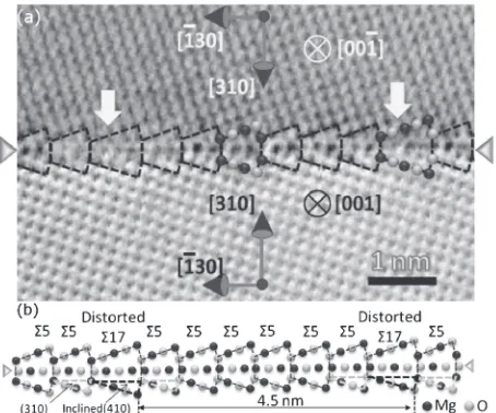
Recently, observations due to high resolutional microscopy combined with theoretical calculations have been con-ducted20­23)and M. Saito et al.24)observed the atomic-scale structures of symmetrical tilt grain boundaries with a bonding angle of 35.3° in a bicrystal of MgO. They demonstrated that the (410)-structural units of­17 are periodically intercalated in between the (310)-structural units of ­5 and recognised such phenomenon as the periodic appearance of displace-ment-shift-complete (DSC) dislocations.

While most of the successful works relied on micro-scopical observations and extensive numerical calculations, we propose a novel method to analyse the structures of symmetrical tilt grain boundaries of simple cubic crystals with the rotation axis of©001ªwith a mathematically evident argument. Sutton et al. gave an algorithm to obtain the arrangement of structural units assuming that the boundary structure can be described by two favoured boundaries as a linear combination of them with coprime integral coefficients and the structure changes as continuously as possible according to the misorientation.3) _{Our approach to describe}

the boundary structure is the converse of their argument. We directly derive the decomposition formula of the©001ªgrain

boundaries and reproduce the previously observed results by the aid of the structural-units model and conventionally-called the O-lattice theory. The ratio of the number of the structural units is precisely given as a corollary.

The O-lattice theory was introduced by W. Bollmann25­29) as a way of generalisations of the coincidence-site-lattice (CSL) theory.30)We utilise the O-lattice as an indicator of the periodicity of the structural units and therefore, it is different from the way Bollmann proposed. In this theory, letL0be a

2-dimensional square lattice and L1, L2 be lattices which

satisfy L_i¼A_iðL₀Þ (i=1, 2) for a non-degenerate linear transformation Ai. LetUðL0Þ denote the unit cell ofL0 and jUðL0Þj denote its area. In what follows, the pair of lattices

ðL0; L1Þ is assumed to be a configuration slightly deviated from the optimal configurationðL0; L2Þ. For the dichromatic pattern18,19) _{of a pair of latticesðL0; L}

iÞ, an O-point a with

respect toAican be expressed by the following basic equation

which can be derived by the Frank-Bilby formula:31­34)

ðIA1

i Þa¼t0; ð1Þ

where I is the identity matrix and t0 is an arbitrary translational vector in L0. From the eq. (1), a is recognized

as the centre of the linear transformationAiin the dichromatic

pattern of ðL0; L_iÞ. In this sense, the O-lattice is a way of generalisation of the CSL since any of the CSL points can be the centre of a rotational transformation. One of the points the O-lattice theory has been criticised is that the choice of Ai

is not unique. However, this ambiguity allows us to choose an appropriate transformation according to the problem. Let

OAiðL0; LiÞdenote the O-lattice ofðL0; LiÞwith respect toAi.

Conversely, given an O-point and the transformation Ai, the

configuration of the lattices around it is recovered. From the eq. (1), one can see that jUðL0Þj=jdetðIA1

i Þj gives the

area of the unit cell of the O-lattice and therefore that

j_detðIA1

i Þjis a sort of the density of O-points as with­

in the CSL theory. Generally, an O-lattice is a super-lattice of the CSL in a CSL configuration if Ai is a rotational

transformation and thus the unit cell of an O-lattice is smaller than that of the CSL. The O-points can be classified in terms of the internal coordinates. Two O-points are equivalent if their internal coordinates coincide, the representatives of which are called the reduced O-points. It can be shown that

+_{Corresponding author, E-mail: kinoue@wpi-aimr.tohoku.ac.jp}

there are two types (resp. four types) of reduced O-points for theðm 1 0Þ-plane wheremis an odd (resp. even) integer ifAi

is a rotational transformation. Table 1 shows the examples of the reduced O-points for the small­’s.

The O-lattice defined above is called the primary O-lattice or simply the O1-lattice. As an alternative, we can also define

a secondary O-lattice or simply an O2-lattice. The O1-lattice OAiðL0; LiÞ can be defined for each i=1, 2. Then the

transformation A1A1

2 maps L2 to L1 and thus the

trans-formation ðIA1 1 Þ

1_ðIA1

2 Þ maps OA2ðL0; L2Þ to OA1ðL0; L1Þ. Letting B¼ ðIA11Þ

1_ðIA1

2 Þ, the O2

-lattice is defined to be the O1-lattice of two O1-lattices with

respect to the transformation B. Namely, an O2-point b is

given by25)

ðIB1_Þb¼t

1; ð2Þ

where t₁ is an arbitrary translational vector in the reference O1-latticeOA2ðL0; L2Þ. The basic equation of the O2-lattice is

also given by

ðIA1A1

2 Þb¼t2; ð3Þ

wheret₂is an arbitrary translational vector of the DSC lattice of ðL0; L2Þ. The O2-lattice is in general a sub-lattice of the

reference O1-lattice. It is expected that the secondary

dislocations (or the DSC dislocations) are introduced into the boundary of the Wigner-Seitz cells of the O2-points under

the assumptions that the deviation of ðL0; L1Þ from the optimal configuration ðL0; L2Þis small enough.28,35,36)

2. Application of the O-Lattice Theory

Wefirst demonstrate the application of the O-lattice theory by focusing on the symmetrical tilt CSL grain boundaries. The termnear CSL37)_{can be defined as a configuration of a}

pair of two lattices which are, in a sense, close to an optimal configuration (a favoured boundary,3)_{or a preferred state}28)_).

Note that the term near CSL can be used even for a CSL configuration with a high­. LetLibe given by the rotation of L0with a rotational transformationRð2ªiÞof the angle of 2ªi

(i=1, 2), respectively. It is assumed that a CSL confi g-uration with a high ­ can be approximated by two of the optimal reference configurations with low ­’s. In this way, the periodicity of grain boundaries can be easily evaluated by the structural-units model.2­5)In this paper, we consider the

ðq p 0Þ-planes. As highlighted in Fig. 1, the structural unit

of symmetricalðq p0Þ-grain boundary can be defined to be a kite-shaped tetragon which is made by gluing a pair of right triangles of a group of atoms at their hypotenuses whose sides in the right angles areqaandpawhereais the average atomic distance. Since a desired resolution around the

boundary may not always be obtained, we take a larger cell enclosing the structural unit defined above. Figure 1 shows the atomic configurations of the (310)-structural units of the ­5 boundary and the (410)-structural units of the ­17 boundary where two latticesL0and L1are superposed. The

CSL boundary is defined by the line passing through the CSL points below which there are points of L0 and above which

there are points ofL1.

If ðL₀; L₁Þ is of a CSL configuration, it holds that

tanª1¼p=q for coprime positive integers p and q. It is

shown that the periodicity of the structural units in the

ðq p 0Þ-plane isp. By takingA¼Rð2ª1Þin the eq. (1), we have

ðIRð₂ª1Þ1_Þ1_¼1

2

1 q=p

q=p 1

: ð₄Þ

By applying the eq. (4) to a translational vectorð0; lÞofL0for

an integerlto obtain the O-points on theðq p0Þ-plane, one can have

ðIRð₂ª1Þ1_Þ1 0 l ¼

l

2

q=p

1

: ð₅Þ

Then the point l=2ðq=p 1 0Þ belongs to the ðq p 0Þ-plane. The CSL points are obtained by the eq. (5) if the parameterl

is divisible by 2p. If l is odd, the first component of the eq. (5) varies while the second component is maintained at 1/2 in terms of the internal coordinates. It is concluded that the internal coordinates in the eq. (5) is periodic and the periodicity can be precisely given by 2p. By drawingvirtual

structural units passing through O1-points alternately, it can

be shown that the periodicity of the structural units is given byp.

In order to validate the above method, we consider the

ð_{22 7 0}Þ-structure as a model case which corresponds to the

misorientation of the angle of 35.300° (tanð35:300=2Þ ’ 7=22) and is a near (310)­5-structure of the angle of 36.869° (tanð36:869=2Þ ’1=3). Figure 2 shows the dichromatic pattern of the ð22 7 0Þ-structure with the unit cells ofL0. It

can be seen that O-points in the virtual structural unit shifts periodically inUðL₀Þ. In the fourth structural unit from the left, onefinds an O-point at the edge ofUðL₀Þwhose internal

Table 1 Examples of reduced O-points for the small­’s ifAiis a rotational transformation.

­ 2ª cotª g.b. plane reduced O-points ­13 22.62° 5 (510) ð0;0Þ,ð1=2;1=2Þ

­17 28.07° 4 (410) ð0;0Þ,ð1=2;1=2Þ,ð0;1=2Þ,ð1=2;0Þ

­5 36.87° 3 (310) ð0;0Þ,ð1=2;1=2Þ

­5 53.13° 2 (210) ð0;0Þ,ð1=2;1=2Þ,ð0;1=2Þ,ð1=2;0Þ

Fig. 1 (a) The (310)-structural units of the­5 boundary and (b) the (410)-structural units of the17boundary. The reference latticeL0, the rotated

coordinates areð0;1=2Þwith respect to the coordinate system of L0. Since the theoretical grain boundary is on the

ð_{22 7 0}Þ-plane the above argument suggests that the

periodicity of the structural units is 7. The deviation of the angle 35.300° identifies this CSL configuration as ­533 which is in between 36.869°(­5) and 28.072°(­17). There-fore this grain boundary can be described by the combination of the (310) and the (410)-planes. The internal coordinates of the eq. (5) becomesð0;1=2Þifl¼7þ14kfor each integerk

which appears not in the ­5 but in the ­17 configuration (Table 1). The decomposition is thus given by the linear combination with integral coefficients of the reference boundaries.3) Namely, it holds that ð22 7 0Þ ¼6ð3 1 0Þ þ

1ð4 1 0Þ, which is viewed as a decomposition of a reciprocal

vector. Once two reference structures are determined appropriately, one can obtain the integral coefficients uniquely for a specific grain boundary. Figure 3 shows an ABF-STEM image of the MgO grain boundary with a bonding angle of 35.3° and a corresponding schematic plot of the structural units, indicating that the periodicity of the structural units is 7 though it can be varied in the presence of impurities.24)

For each m¼2;3;4;5;. . ., let p/q be a rational number for coprime positive integers p and q with 1=m < p=q < 1=ðm1Þ. Since theðm1 0Þand theðm1 1 0Þ-planes can be the reference structures for the ðq p 0Þ-plane, the first decomposition rule is summarised as follows:

ðq p 0Þ ¼n1ðm 1 0Þ þn2ðm1 1 0Þ; ð6Þ

where n1¼q ðm1Þp and n2¼ qþmp are positive integers. Similar equations were discussed by A. A. Levi

et al.15) _{and by Sutton et al.}38) _{to describe the arrangement}

of the structural units. Note that n₁þn₂ ¼p defines the periodicity of the structural units. It holds that n1> n2 if the ðq p0Þ-plane is close to the ðm1 0Þ-plane i.e. 1=m <

p=q <2=ð2m1Þ and n1< n2 holds otherwise where

2=ð2m1Þ is the harmonic average of 1/mand1=ðm1Þ. The eq. (6) not only agrees with the microscopical observation by Saito et al.24)but successfully generalise the results of theoretical calculations by G. J. Wang et al.,8,9) relatively recent results by S. P. Chen et al.,14)and most of the experimental results by N. D. Browninget al.16)It should be remarked that our argument goes in the opposite direction of Sutton’s.3)_{Although we only focus on the nearð3 1 0Þ­5}

grain boundaries in this paper, the formula can be valid in more general cases which will be discussed further. Readers can refer to the decomposition table of the (qp0)-planes

around­5ð2ª¼36:869Þwithp<10 presented in Table 2 and more detailed cases for largerp’s in the appendix.

We may assume that the periodicity p is smaller than 10 sincenature might not prefer a long periodicity. Then it can be shown that the numerators of the irreducible rational numbers in between 1/mand 1=ðm1Þ which are smaller than 10 form a mirror-symmetric sequencefp_lg29_l¼1:

1;9;8;7;6;5;9;4;7;3;8;5;7;9;2;

9;7;5;8;3;7;4;9;5;6;7;8;9;1: ð7Þ

For instance, irreducible rational numbers in between 1/4 and 1/3 whose numerators are less than 10 can be given by 1/4, 9/35, 8/31, 7/27, 6/23, 5/19, 9/34, 4/15, 7/26, 3/11, 8/29, 5/18, 7/25, 9/32, 2/7, 9/31, 7/24, 5/17, 8/27, 3/10, 7/23, 4/13, 9/29, 5/16, 6/19, 7/22, 8/25, 9/28, 1/3. Therefore, if p1¼1 and p29¼1 correspond to the (410)-plane with 28.072° and the (310)-plane with 36.869°, respectively,

p26¼₇ corresponds to the ð22 7 0Þ-plane with 2ª= 35.300°. It is observed that pl ¼pl1þplþ1 holds for l¼₂;7;9;11;14;16;19;21;23;28 (underlined) correspond-ing to the decomposition of a periodicitypltopl1andplþ1

which can be also shown by the periodicity of the O-points. Let q_l be the denominator that corresponds to p_l. We can now propose the second decomposition rule as follows. If it satisfies thatp_l¼p_l1þplþ1, the eq. (6) can be modified to

ðql pl 0Þ ¼ ½nlð1Þ1ðm 1 0Þ þn

ð2Þ

l1ðm1 1 0Þ

þ ½nð1Þ

lþ1ðm1 0Þ þn

ð2Þ

lþ1ðm1 1 0Þ; ð8Þ

wherenð_liÞ¼nð_liÞ₁þn_lði_þÞ₁ði¼1;2Þsatisfying thatnð_L1Þ ¼q_L

ðm₁ÞpL and nðL2Þ¼ qLþmpLðL¼l1; l; lþ1Þ. For

instance, the ð32 9 0Þ-structure corresponding to the misor-ientation angle of 31.417° decomposes into 5ð4 1 0Þ þ

4ð3 1 0Þ according to the eq. (6). On the other hand, since

9/32 is in between 7/25 and 2/7, theð32 9 0Þ-structure can be composed of theð25 7 0Þand theð7 2 0Þ-structures, each of which decomposes into4ð4 1 0Þ þ3ð3 1 0Þandð4 1 0Þ þ

ð3 1 0Þ, respectively, corresponding to the decomposition of

the periodicity 9 into 7 and 2. It can be easily seen in Table 2. Note that theðm 1 0Þ-plane can be decomposed into smaller indices whenmis greater than 4.

Fig. 2 Theð22 7 0Þ-structure with virtual structural units. The reference latticeL0, the rotated latticeL2of the angle of 35.30° and theO1-lattice

OðL0; L2Þare presented, indicating thatO1-point is shifted in the unit cell

ofL0. After the relaxation, the virtual structural units are transformed to

(possibly deformed) six (310)-units and one (410)-unit.

The findings by Saito et al.24) can be interpreted from a viewpoint of the O2-lattice. Figure 4 shows the dichromatic

pattern of the ð22 7 0Þ-structure with the virtual structural units in which the line passing through the CSL points indicates the ð22 7 0Þ-boundary connecting two CSL O2

-points and the diagonal lines are the boundary of the Wigner-Seitz cells of O2-points. Given cotª2 is an odd integer,

A1¼Rð2ª1Þ and A2¼Rð2ª2Þ in the eqs. (1) and (3), the

area of the unit cells of the O1-lattice ofðL0; L2Þand the O2

-lattice of ðL0; L1; L2Þ can be given by VO₁¼1=4 sin2ª2,

VO2¼sin

2_{ª1=2 sin}2_{ª, respectively, where ª¼ª2ª1.}

Since their unit cells are square, the ratio of the length of the sidelO₁ andlO₂ can be given by

lO2

lO1 ¼

ffiffiffi

2 p

jcotª1cotª2j: ð9Þ

By taking cotª1¼22=7ð2ª1¼35:30Þ and cotª2¼ 3ð2ª2¼36:87Þ, the value of the eq. (9) is given by 7pffiffiffi2. The length of the diagonal line of the unit O2-cell is therefore

estimated to be14lO1, indicating that there are 15 O1-points

that are arrayed regularly on the CSL boundary in Fig. 4. The theory of the O2-lattice suggests that a DSC dislocation can

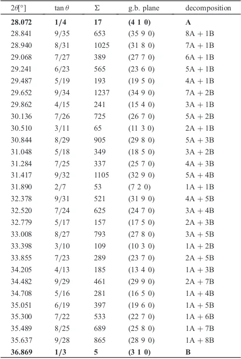
Table 2 The decomposition table for the (qp0)-plane around ­5 (2ª= 36.869°) with p<10 is presented. The reference configurations are denoted by A¼ ð4 1 0Þ, B¼ ð3 1 0Þ and C¼ ð2 1 0Þ which are represented in boldstyle. The second rule of decomposition in the eq. (8) is observed.

2ª[°] tanª ­ g.b. plane decomposition

28.072 1/4 17 (4 1 0) A

28.841 9/35 653 (35 9 0) 8A+1B 28.940 8/31 1025 (31 8 0) 7A+1B 29.068 7/27 389 (27 7 0) 6A+1B 29.241 6/23 565 (23 6 0) 5A+1B 29.487 5/19 193 (19 5 0) 4A+1B 29.652 9/34 1237 (34 9 0) 7A+2B 29.862 4/15 241 (15 4 0) 3A+1B 30.136 7/26 725 (26 7 0) 5A+2B 30.510 3/11 65 (11 3 0) 2A+1B 30.844 8/29 905 (29 8 0) 5A+3B 31.048 5/18 349 (18 5 0) 3A+2B 31.284 7/25 337 (25 7 0) 4A+3B 31.417 9/32 1105 (32 9 0) 5A+4B 31.890 2/7 53 (7 2 0) 1A+1B 32.378 9/31 521 (31 9 0) 4A+5B 32.520 7/24 625 (24 7 0) 3A+4B 32.779 5/17 157 (17 5 0) 2A+3B 33.008 8/27 793 (27 8 0) 3A+5B 33.398 3/10 109 (10 3 0) 1A+2B 33.855 7/23 289 (23 7 0) 2A+5B 34.205 4/13 185 (13 4 0) 1A+3B 34.482 9/29 461 (29 9 0) 2A+7B 34.708 5/16 281 (16 5 0) 1A+4B 35.051 6/19 397 (19 6 0) 1A+5B 35.300 7/22 533 (22 7 0) 1A+6B 35.489 8/25 689 (25 8 0) 1A+7B 35.637 9/28 865 (28 9 0) 1A+8B

36.869 1/3 5 (3 1 0) B

Continued on next column:

Continued:

2ª[°] tanª ­ g.b. plane decomposition

36.869 1/3 5 (3 1 0) B

38.186 9/26 757 (26 9 0) 8B+1C 38.358 8/23 593 (23 8 0) 7B+1C 38.580 7/20 449 (20 7 0) 6B+1C 38.880 6/17 325 (17 6 0) 5B+1C 39.307 5/14 221 (14 5 0) 4B+1C 39.597 9/25 353 (25 9 0) 7B+2C 39.966 4/11 137 (11 4 0) 3B+1C 40.449 7/19 205 (19 7 0) 5B+2C 41.112 3/8 73 (8 3 0) 2B+1C 41.708 8/21 505 (21 8 0) 5B+3C 42.075 5/13 97 (13 5 0) 3B+2C 42.501 7/18 373 (18 7 0) 4B+3C 42.741 9/23 305 (23 9 0) 5B+4C 43.602 2/5 29 (5 2 0) 1B+1C 44.498 9/22 565 (22 9 0) 4B+5C 44.760 7/17 169 (17 7 0) 3B+4C 45.239 5/12 169 (12 5 0) 2B+3C 45.667 8/19 425 (19 8 0) 3B+5C 46.397 3/7 29 (7 3 0) 1B+2C 47.258 7/16 305 (16 7 0) 2B+5C 47.924 4/9 97 (9 4 0) 1B+3C 48.455 9/20 481 (20 9 0) 2B+7C 48.887 5/11 73 (11 5 0) 1B+4C 49.550 6/13 205 (13 6 0) 1B+5C 50.033 7/15 137 (15 7 0) 1B+6C 50.402 8/17 353 (17 8 0) 1B+7C 50.692 9/19 221 (19 9 0) 1B+8C

53.130 1/2 5 (2 1 0) C

Fig. 4 The dichromatic pattern of the ð22 7 0Þ-structure with virtual structural units. The reference latticeL0, the rotated latticeL1of angle of

35.30°, the O1-lattice OðL0; L1Þand the O2-lattice are presented. The

diagonal lines crossing perpendicularly shows the boundary of the Wigner-Seitz cells of O2-points. In the fourth structural unit from the left,

be introduced at the intersection of the CSL boundary and the boundary of the Wigner-Seitz cells of the O2-lattice. It occurs

at the middle of the array of 15 O1-points where the internal

coordinates of it are ð0;1=2Þ. One of the atoms around the point should be shifted by the DSC Burgers vector close to

½_{3 1 0}=10 of the ­5 configuration through relaxation in

order to localise the misfit.

3. Conclusion

We have applied the O-lattice theory to analyse the structures of symmetrical tilt grain boundaries of cubic crystals with the rotation axis©001ªand successfully derived a decomposition formula for symmetrical tilt near ­5 grain boundaries. We provide a convincing theoretical interpreta-tion for the observed structures of a near­5 grain boundary in MgO both from the structural-units model and the theory of the secondary O-lattice. The established theoretical formulae help to elucidate the fundamental structural relationship in a grain boundary and provide an approach for understanding structures of random grain boundaries.

Acknowledgements

The authors are grateful to Prof. Hideo Yoshinaga and Prof. Wenzheng Zhang for valuable discussions. This work is supported in part by Nippon Steel & Sumitomo Metal Corporation, the Elements Strategy Initiative for Structural Materials (ESISM) by the MEXT of Japan, the JSPS Grant-in-Aid for Scientific Research on Innovative Areas “Nano Informatics” (Grant No. 251006005), the Grant-in-Aid for Young Scientists (A) (grant no. 24686069), NSFC (grant no. 11332013) and, JSPS and CAS under the Japan-China Scientific Cooperation Program.

REFERENCES

1) G. H. Bishop and B. Chalmers:Scr. Metall.2(1968) 133­139.

2) A. P. Sutton and V. Vitek: Acta Metall.14(1980) 129­132. 3) A. P. Sutton and V. Vitek:Philos. Trans. R. Soc. Lond. A309(1983)

1­36.

4) A. P. Sutton and V. Vitek:Philos. Trans. R. Soc. Lond. A309(1983) 37­54.

5) A. P. Sutton and V. Vitek:Philos. Trans. R. Soc. Lond. A309(1983) 55­68.

6) R. C. Pond, D. A. Smith and V. Vitek:Acta Metall.27(1979) 235­241.

7) R. W. Balluffiand P. D. Bristowe:Surf. Sci.144(1984) 28­43.

8) G.-J. Wang, A. P. Sutton and V. Vitek:Acta Metall.32(1984) 1093­ 1104.

9) G.-J. Wang and V. Vitek:Acta Metall.34(1986) 951­960.

10) R. C. Pond:Proc. R. Soc. A357(1977) 471­483.

11) R. C. Pond and V. Vitek:Proc. R. Soc. A357(1977) 453­470.

12) V. Vitek, D. A. Smith and R. C. Pond:Philos. Mag.41(1980) 649­663.

13) M. Kohyama:Phys. Stat. Sol. (b)141(1987) 71­83.

14) S. P. Chen, D. J. Srolovitz and A. F. Voter:J. Mat. Res.4(1989) 62­77.

15) A. A. Levi, D. A. Smith and J. T. Wetzel:J. Appl. Phys.69(1991) 2048­2056.

16) N. D. Browning, S. J. Pennycook, M. F. Chisholm, M. M. McGibbon and A. J. McGibbon:Interface Sci.2(1995) 397­423.

17) A. P. Sutton and R. W. Balluffi:Interfaces in Crystalline Materials, (Clarendon Press, Oxford, 1995).

18) R. C. Pond and W. Bollmann: Philos. Trans. R. Soc. Lond. A292 (1979) 449­472.

19) R. C. Pond and D. S. Vlachavas:Proc. R. Soc. A386(1983) 95­143.

20) C. Schmidt, M. W. Finnis, F. Ernst and V. Vitek:Philos. Mag. A77 (1998) 1161­1184.

21) N. Shibata, F. Oba, T. Yamamoto and Y. Ikuhara: Philos. Mag.84 (2004) 2381­2415.

22) M. Imaeda, T. Mizoguchi, Y. Sato, H.-S. Lee, S. D. Findlay, N. Shibata, T. Yamamoto and Y. Ikuhara:Phys. Rev. B78(2008) 245320.

23) H. Hojo, T. Mizoguchi, H. Ohta, S. D. Findlay, N. Shibata, T. Yamamoto and Y. Ikuhara:Nano Lett.10(2010) 4668­4672.

24) M. Saito, Z. Wang, S. Tsukimoto and Y. Ikuhara:J. Mater. Sci.48 (2013) 5470­5474.

25) W. Bollmann: Crystal Defects and Crystalline Interfaces, (Springer-Verlag, Berlin, 1970).

26) W. Bollmann:Surf. Sci.31(1972) 1­11.

27) R. C. Pond and D. A. Smith: Int. Met. Rev.June(1976) 61­74. 28) W. Bollmann:Crystal Lattices, Interfaces, Matrices, published by the

author, Geneva, (1982).

29) C. Solenthaler and W. Bollmann:Mater. Sci. Eng.81(1986) 35­49.

30) S. Ranganathan:Acta Cryst.21(1966) 197­199.

31) F. C. Frank: Symposium on the Plastic Deformation of Crystalline Solids, (1950) pp. 150­154.

32) B. A. Bilby:Report on the Conference on Defects in Crystalline Solids, (1955) pp. 124­133.

33) J. W. Christian:The Theory of Transformations in Metals and Alloys, 3rd ed., (Pergamon, Oxford, 2002).

34) J. P. Hirth, R. C. Pond, R. G. Hoagland, X.-Y. Liu and J. Wang:Prog. Mat. Sci.58(2013) 749­823.

35) Z.-Z. Shi, F.-Z. Dai, M. Zhang, X.-F. Gu and W.-Z. Zhang:Metall. Mat. Trans. A44(2013) 2478­2486.

36) W.-Z. Zhang:Metall. Mat. Trans. A44(2013) 4513­4531.

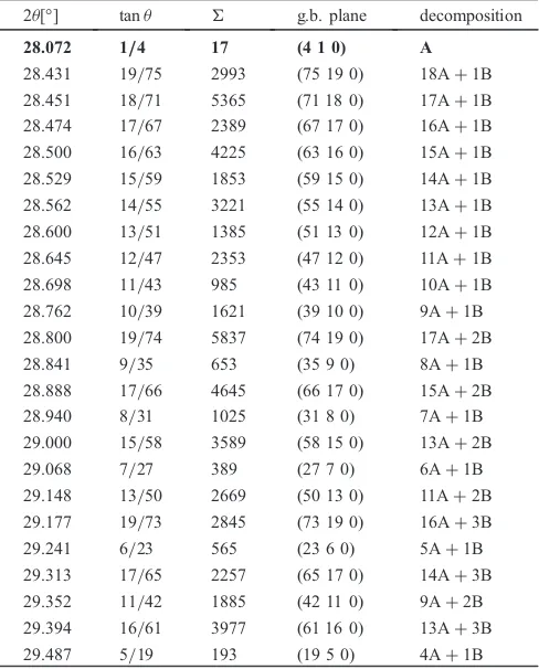
37) G. A. Bruggeman, G. H. Bishop and W. H. Hartt:The Nature and Behavior of Grain Boundaries, (Plenum Press, New York, 1972) pp. 83­122.

38) A. P. Sutton:Prog. Mat. Sci.36(1992) 167­202. Appendix

Table A.1 The decomposition table for the ðq p0Þ-plane around ­5

ð2ª¼36:869Þwithp <20is presented. The reference configurations are denoted by A¼ ð4 1 0Þ, B¼ ð3 1 0Þ and C¼ ð2 1 0Þ which are represented in boldstyle.

2ª[°] tanª ­ g.b. plane decomposition

28.072 1/4 17 (4 1 0) A

28.431 19/75 2993 (75 19 0) 18A+1B 28.451 18/71 5365 (71 18 0) 17A+1B 28.474 17/67 2389 (67 17 0) 16A+1B 28.500 16/63 4225 (63 16 0) 15A+1B 28.529 15/59 1853 (59 15 0) 14A+1B 28.562 14/55 3221 (55 14 0) 13A+1B 28.600 13/51 1385 (51 13 0) 12A+1B 28.645 12/47 2353 (47 12 0) 11A+1B 28.698 11/43 985 (43 11 0) 10A+1B 28.762 10/39 1621 (39 10 0) 9A+1B 28.800 19/74 5837 (74 19 0) 17A+2B 28.841 9/35 653 (35 9 0) 8A+1B 28.888 17/66 4645 (66 17 0) 15A+2B 28.940 8/31 1025 (31 8 0) 7A+1B 29.000 15/58 3589 (58 15 0) 13A+2B 29.068 7/27 389 (27 7 0) 6A+1B 29.148 13/50 2669 (50 13 0) 11A+2B 29.177 19/73 2845 (73 19 0) 16A+3B 29.241 6/23 565 (23 6 0) 5A+1B 29.313 17/65 2257 (65 17 0) 14A+3B 29.352 11/42 1885 (42 11 0) 9A+2B 29.394 16/61 3977 (61 16 0) 13A+3B 29.487 5/19 193 (19 5 0) 4A+1B

Continued:

2ª[°] tanª ­ g.b. plane decomposition 29.565 19/72 5545 (72 19 0) 15A+4B 29.593 14/53 3005 (53 14 0) 11A+3B 29.652 9/34 1237 (34 9 0) 7A+2B 29.717 13/49 1285 (49 13 0) 10A+3B 29.751 17/64 4385 (64 17 0) 13A+4B 29.862 4/15 241 (15 4 0) 3A+1B 29.963 19/71 2701 (71 19 0) 14A+5B 29.990 15/56 3361 (56 15 0) 11A+4B 30.036 11/41 901 (41 11 0) 8A+3B 30.075 18/67 4813 (67 18 0) 13A+5B 30.136 7/26 725 (26 7 0) 5A+2B 30.202 17/63 2129 (63 17 0) 12A+5B 30.248 10/37 1469 (37 10 0) 7A+3B 30.308 13/48 2473 (48 13 0) 9A+4B 30.345 16/59 3737 (59 16 0) 11A+5B 30.371 19/70 5261 (70 19 0) 13A+6B 30.510 3/11 65 (11 3 0) 2A+1B 30.666 17/62 4133 (62 17 0) 11A+6B 30.700 14/51 2797 (51 14 0) 9A+5B 30.752 11/40 1721 (40 11 0) 7A+4B 30.791 19/69 2561 (69 19 0) 12A+7B 30.844 8/29 905 (29 8 0) 5A+3B 30.922 13/47 1189 (47 13 0) 8A+5B 30.957 18/65 4549 (65 18 0) 11A+7B 31.048 5/18 349 (18 5 0) 3A+2B 31.145 17/61 2005 (61 17 0) 10A+7B 31.185 12/43 1993 (43 12 0) 7A+5B 31.221 19/68 4985 (68 19 0) 11A+8B 31.284 7/25 337 (25 7 0) 4A+3B 31.359 16/57 3505 (57 16 0) 9A+7B 31.417 9/32 1105 (32 9 0) 5A+4B 31.502 11/39 821 (39 11 0) 6A+5B 31.561 13/46 2285 (46 13 0) 7A+6B 31.605 15/53 1517 (53 15 0) 8A+7B 31.638 17/60 3889 (60 17 0) 9A+8B 31.664 19/67 2425 (67 19 0) 10A+9B 31.890 2/7 53 (7 2 0) 1A+1B 32.119 19/66 4717 (66 19 0) 9A+10B 32.147 17/59 1885 (59 17 0) 8A+9B 32.181 15/52 2929 (52 15 0) 7A+8B 32.226 13/45 1097 (45 13 0) 6A+7B 32.288 11/38 1565 (38 11 0) 5A+6B 32.378 9/31 521 (31 9 0) 4A+5B 32.440 16/55 3281 (55 16 0) 7A+9B 32.520 7/24 625 (24 7 0) 3A+4B 32.588 19/65 2293 (65 19 0) 8A+11B 32.627 12/41 1825 (41 12 0) 5A+7B 32.672 17/58 3653 (58 17 0) 7A+10B 32.779 5/17 157 (17 5 0) 2A+3B 32.880 18/61 4045 (61 18 0) 7A+11B 32.920 13/44 2105 (44 13 0) 5A+8B 33.008 8/27 793 (27 8 0) 3A+5B 33.069 19/64 4457 (64 19 0) 7A+12B 33.114 11/37 745 (37 11 0) 4A+7B 33.174 14/47 2405 (47 14 0) 5A+9B 33.213 17/57 1769 (57 17 0) 6A+11B

Continued on next column:

Continued:

2ª[°] tanª ­ g.b. plane decomposition 33.398 3/10 109 (10 3 0) 1A+2B 33.565 19/63 2165 (63 19 0) 6A+13B 33.596 16/53 3065 (53 16 0) 5A+11B 33.642 13/43 1009 (43 13 0) 4A+9B 33.716 10/33 1189 (33 10 0) 3A+7B 33.773 17/56 3425 (56 17 0) 5A+12B 33.855 7/23 289 (23 7 0) 2A+5B 33.932 18/59 3805 (59 18 0) 5A+13B 33.981 11/36 1417 (36 11 0) 3A+8B 34.041 15/49 1313 (49 15 0) 4A+11B 34.075 19/62 4205 (62 19 0) 5A+14B 34.205 4/13 185 (13 4 0) 1A+3B 34.351 17/55 1657 (55 17 0) 4A+13B 34.397 13/42 1933 (42 13 0) 3A+10B 34.482 9/29 461 (29 9 0) 2A+7B 34.562 14/45 2221 (45 14 0) 3A+11B 34.601 19/61 2041 (61 19 0) 4A+15B 34.708 5/16 281 (16 5 0) 1A+4B 34.835 16/51 2857 (51 16 0) 3A+13B 34.894 11/35 673 (35 11 0) 2A+9B 34.949 17/54 3205 (54 17 0) 3A+14B 35.051 6/19 397 (19 6 0) 1A+5B 35.142 19/60 3961 (60 19 0) 3A+16B 35.184 13/41 925 (41 13 0) 2A+11B 35.300 7/22 533 (22 7 0) 1A+6B 35.400 15/47 1217 (47 15 0) 2A+13B 35.489 8/25 689 (25 8 0) 1A+7B 35.567 17/53 1549 (53 17 0) 2A+15B 35.637 9/28 865 (28 9 0) 1A+8B 35.700 19/59 1921 (59 19 0) 2A+17B 35.757 10/31 1061 (31 10 0) 1A+9B 35.855 11/34 1277 (34 11 0) 1A+10B 35.938 12/37 1513 (37 12 0) 1A+11B 36.008 13/40 1769 (40 13 0) 1A+12B 36.068 14/43 2045 (43 14 0) 1A+13B 36.120 15/46 2341 (46 15 0) 1A+14B 36.166 16/49 2657 (49 16 0) 1A+15B 36.207 17/52 2993 (52 17 0) 1A+16B 36.243 18/55 3349 (55 18 0) 1A+17B 36.276 19/58 3725 (58 19 0) 1A+18B

36.869 1/3 5 (3 1 0) B

37.482 19/56 3497 (56 19 0) 18B+1C 37.517 18/53 3133 (53 18 0) 17B+1C 37.556 17/50 2789 (50 17 0) 16B+1C 37.599 16/47 2465 (47 16 0) 15B+1C 37.649 15/44 2161 (44 15 0) 14B+1C 37.706 14/41 1877 (41 14 0) 13B+1C 37.772 13/38 1613 (38 13 0) 12B+1C 37.849 12/35 1369 (35 12 0) 11B+1C 37.940 11/32 1145 (32 11 0) 10B+1C 38.051 10/29 941 (29 10 0) 9B+1C 38.115 19/55 1693 (55 19 0) 17B+2C 38.186 9/26 757 (26 9 0) 8B+1C 38.267 17/49 1345 (49 17 0) 15B+2C 38.358 8/23 593 (23 8 0) 7B+1C 38.461 15/43 1037 (43 15 0) 13B+2C

Continued:

2ª[°] tanª ­ g.b. plane decomposition 38.580 7/20 449 (20 7 0) 6B+1C 38.717 13/37 769 (37 13 0) 11B+2C 38.769 19/54 3277 (54 19 0) 16B+3C 38.880 6/17 325 (17 6 0) 5B+1C 39.004 17/48 2593 (48 17 0) 14B+3C 39.073 11/31 541 (31 11 0) 9B+2C 39.146 16/45 2281 (45 16 0) 13B+3C 39.307 5/14 221 (14 5 0) 4B+1C 39.444 19/53 1585 (53 19 0) 15B+4C 39.493 14/39 1717 (39 14 0) 11B+3C 39.597 9/25 353 (25 9 0) 7B+2C 39.710 13/36 1465 (36 13 0) 10B+3C 39.770 17/47 1249 (47 17 0) 13B+4C 39.966 4/11 137 (11 4 0) 3B+1C 40.143 19/52 3065 (52 19 0) 14B+5C 40.190 15/41 953 (41 15 0) 11B+4C 40.272 11/30 1021 (30 11 0) 8B+3C 40.341 18/49 2725 (49 18 0) 13B+5C 40.449 7/19 205 (19 7 0) 5B+2C 40.565 17/46 2405 (46 17 0) 12B+5C 40.646 10/27 829 (27 10 0) 7B+3C 40.752 13/35 697 (35 13 0) 9B+4C 40.819 16/43 2105 (43 16 0) 11B+5C 40.865 19/51 1481 (51 19 0) 13B+6C 41.112 3/8 73 (8 3 0) 2B+1C 41.390 17/45 1157 (45 17 0) 11B+6C 41.451 14/37 1565 (37 14 0) 9B+5C 41.544 11/29 481 (29 11 0) 7B+4C 41.613 19/50 2861 (50 19 0) 12B+7C 41.708 8/21 505 (21 8 0) 5B+3C 41.849 13/34 1325 (34 13 0) 8B+5C 41.911 18/47 2533 (47 18 0) 11B+7C 42.075 5/13 97 (13 5 0) 3B+2C 42.249 17/44 2225 (44 17 0) 10B+7C 42.322 12/31 1105 (31 12 0) 7B+5C 42.388 19/49 1381 (49 19 0) 11B+8C 42.501 7/18 373 (18 7 0) 4B+3C 42.635 16/41 1937 (41 16 0) 9B+7C 42.741 9/23 305 (23 9 0) 5B+4C 42.895 11/28 905 (28 11 0) 6B+5C 43.002 13/33 629 (33 13 0) 7B+6C 43.081 15/38 1669 (38 15 0) 8B+7C 43.142 17/43 1069 (43 17 0) 9B+8C 43.190 19/48 2665 (48 19 0) 10B+9C 43.602 2/5 29 (5 2 0) 1B+1C 44.022 19/47 1285 (47 19 0) 9B+10C 44.072 17/42 2053 (42 17 0) 8B+9C 44.135 15/37 797 (37 15 0) 7B+8C 44.218 13/32 1193 (32 13 0) 6B+7C 44.332 11/27 425 (27 11 0) 5B+6C 44.498 9/22 565 (22 9 0) 4B+5C 44.612 16/39 1777 (39 16 0) 7B+9C 44.760 7/17 169 (17 7 0) 3B+4C 44.885 19/46 2477 (46 19 0) 8B+11C 44.958 12/29 985 (29 12 0) 5B+7C 45.041 17/41 985 (41 17 0) 7B+10C

Continued on next column:

Continued:

2ª[°] tanª ­ g.b. plane decomposition 45.239 5/12 169 (12 5 0) 2B+3C 45.428 18/43 2173 (43 18 0) 7B+11C 45.501 13/31 565 (31 13 0) 5B+8C 45.667 8/19 425 (19 8 0) 3B+5C 45.781 19/45 1193 (45 19 0) 7B+12C 45.864 11/26 797 (26 11 0) 4B+7C 45.977 14/33 1285 (33 14 0) 5B+9C 46.050 17/40 1889 (40 17 0) 6B+11C 46.397 3/7 29 (7 3 0) 1B+2C 46.711 19/44 2297 (44 19 0) 6B+13C 46.770 16/37 1625 (37 16 0) 5B+11C 46.857 13/30 1069 (30 13 0) 4B+9C 46.997 10/23 629 (23 10 0) 3B+7C 47.104 17/39 905 (39 17 0) 5B+12C 47.258 7/16 305 (16 7 0) 2B+5C 47.405 18/41 2005 (41 18 0) 5B+13C 47.498 11/25 373 (25 11 0) 3B+8C 47.611 15/34 1381 (34 15 0) 4B+11C 47.677 19/43 1105 (43 19 0) 5B+14C 47.924 4/9 97 (9 4 0) 1B+3C 48.204 17/38 1733 (38 17 0) 4B+13C 48.291 13/29 505 (29 13 0) 3B+10C 48.455 9/20 481 (20 9 0) 2B+7C 48.609 14/31 1157 (31 14 0) 3B+11C 48.682 19/42 2125 (42 19 0) 4B+15C 48.887 5/11 73 (11 5 0) 1B+4C 49.134 16/35 1481 (35 16 0) 3B+13C 49.247 11/24 697 (24 11 0) 2B+9C 49.353 17/37 829 (37 17 0) 3B+14C 49.550 6/13 205 (13 6 0) 1B+5C 49.727 19/41 1021 (41 19 0) 3B+16C 49.809 13/28 953 (28 13 0) 2B+11C 50.033 7/15 137 (15 7 0) 1B+6C 50.229 15/32 1249 (32 15 0) 2B+13C 50.402 8/17 353 (17 8 0) 1B+7C 50.555 17/36 1585 (36 17 0) 2B+15C 50.692 9/19 221 (19 9 0) 1B+8C 50.815 19/40 1961 (40 19 0) 2B+17C 50.926 10/21 541 (21 10 0) 1B+9C 51.119 11/23 325 (23 11 0) 1B+10C 51.282 12/25 769 (25 12 0) 1B+11C 51.419 13/27 449 (27 13 0) 1B+12C 51.538 14/29 1037 (29 14 0) 1B+13C 51.641 15/31 593 (31 15 0) 1B+14C 51.732 16/33 1345 (33 16 0) 1B+15C 51.813 17/35 757 (35 17 0) 1B+16C 51.884 18/37 1693 (37 18 0) 1B+17C 51.948 19/39 941 (39 19 0) 1B+18C