Optimization of Vacuum Hybrid Welding Process Parameters for YG8 Cemented Carbide and 42CrMo Steel Using Artificial Neural Networks

Optimization of Vacuum Hybrid Welding Process Parameters

for YG8 Cemented Carbide and 42CrMo Steel

Using Arti

fi

cial Neural Networks

Wan-chang Sun

, Pei Zhang, Han-jun Wei, Chun-yu Miao and Kun Zhao

College of Materials Science & Engineering, Xi’an University of Science & Technology, Shaanxi 710054, China

The mechanical properties of the joint of YG8 cemented carbide and 42CrMo steel were studied by using CuZnNifiller metal in the vacuum hybrid welding. The parameters for optimizing the shear strength of joints were selected by orthogonal experiment, mainly including the brazing temperature, brazing time, diffusion temperature, holding time and diffusion pressure. The artificial neural network technique is a very practical tool for predicting the controllable parameters in the non-linear model. BP (Back Propagation) neural network was established under the environment of MATLAB software to simulate and predict designed process parameters. Thus, the optimal parameters were predicted by BP neural network and validated by experiments. The results show that the proposed BP model can obtain a non-linear relationship between the mechanical properties and process parameters. The predicted values are in good agreement with the experiments with the relative error of

¹0.2458%and the mean square error of 0.052%. The optimal parameters of BP neural network were obtained at brazing temperature (A) of 1045°C, brazing time (B) of 15 min, diffusion temperature (C) of 750°C, holding time (D) of 40 min and diffusion pressure (E) of 8 MPa, and the prepared joints showed the better mechanical properties like glossy surface, no apparent deformation, uniform brazing region and good adhesive interface, etc. [doi:10.2320/matertrans.M2015003]

(Received January 6, 2015; Accepted May 21, 2015; Published July 3, 2015)

Keywords: YG8/42CrMo welding joint, vacuum hybrid welding, shear strength, back propagation (BP) neural network, orthogonal experiment

1. Introduction

The welding is one of the important bonding technology in the modern manufacturing industry. Many non-linear prob-lems, which should be non-directly solved with mathematical models, are existed in welding process. Artificial neural network (ANN) modeling is mainly applied very successfully in non-linear system for identification, prediction and simulation, and it has the ability to simulate the non-linear processes about the structure and function of organism. ANN is essentially a large-scale continuous nonlinear time-dynamic system, it shows some characteristics, namely, parallel processing, distributed storage, self-learning and adaptive ability, high fault tolerance, and so forth. The computational nature of ANN can be concluded as state mapping and transformation. ANN modeling can be further divided into feed-forward neural networks and feedback-type neural networks1) _{to better adapt to the development of} science, technology, economy and society. BP (Back Propagation),2)_{which reflects the essence and perfect content,} is a core part of feed-forward neural networks. As well as possessing strong self-learning, organizational, fault-tolerant, self-healing, pattern recognition and retrieval capability,3) BP possesses parallel processing capabilities and a good approximation of non-linear mapping performance.4­8) Therefore, it is widely applied in various fields to deal with complex non-linear problems. BP also shows a bright future for the development and application in material processing.

Vacuum welding furnace could be used to avoid some shortcomings of flame brazing and induction brazing like uneven heating, easy oxidized, etc., so it has been gradually widely applied in bonging between cemented carbides and steels. Sun and Miao proposed and developed a new welding method namely vacuum hybrid welding technology which is

conducted in the vacuum environment, by combining the complementary advantages of the vacuum brazing and vacuum diffusion welding, in order to overcome the short-comings of vacuum brazing and vacuum diffusion welding.9) According to the characteristics of brazing and diffusion welding, the vacuum hybrid welding is expected to have the following characteristics: (1) The welding joints is smooth, with small changes in the mechanical properties, and the general deformation is smaller; (2) This hybrid welding technology could be used for a variety of dissimilar materials, and there are no severe restrictions on the thickness of the workpieces; (3) Phenomenon like oxidation, carburization, decarburization and pollution deterioration will not occur during the welding process; (4) The welding workpieces could be heated evenly, with low residual stress, high welding strength and small deformation after welding; (5) The welding area is of negative pressure, and it is beneficial for the effective release of volatile impurities, thus ensuring the intrinsic performance of the matrix materials; (6) Oxide coatings would not form during the vacuum hybrid welding, so it is not needed to clean slags and spatters after welding, thus greatly improving the working conditions.

This work was to establish a non-linear model for welding YG8 cemented carbide and 42CrMo steel in vacuum hybrid welding with Matlab software under the orthogonal experi-ment, and hence to predict welding parameters using a neural networked technique, because the welding process was a strong non-linear and parameter interconnected process. The welding parameters, including the brazing temperature, brazing time, diffusion temperature, holding time and diffusion pressure were selected as changeable factors while the shear strength10) _{of joint was the} investigation targets. The results show that the welding parameters of YG8 cemented carbide and 42CrMo steel can be predicted and optimized comprehensively by using BP neural network.

+_{Corresponding author, E-mail: sunwanchang@tsinghua.org.cn}

2. Experiments

Vacuum hybrid welding, which includes the techniques of brazing and diffusion welding, was used to avoiding the shortcomings including uneven heating and the susceptible ability to be oxidized. In vacuum environment, solder will be melted and infiltrated into the weld surface when work-pieces and filler metals are heated to just slightly higher than the melting temperature of the solder, with the solderflowing and spreading along the seams by capillary action. Then the alloy layer was formed due to the mutual solution-diffusion and wetting of welding metal and brazingfiller metal. The work-pieces were also pressurized by means of thermal insulation when temperature was below the melting point of the solder. Eventually, the hybrid welding joints were achieved when cooled to the room temperature.

2.1 Experimental materials and equipment

YG8 cemented carbide and 42CrMo steel were regarded as the research object of this work, which were performed at the ZRK-45 vacuum brazing furnace with the pure Ni (60 µm in thickness) for the middle layer material under the vacuum degree of 1©10¹1Pa. The processing diagram of hybrid welding is shown in Fig. 1.

The shear strength of the joints was considered as the evaluating indicator of the mechanical properties, and the joints were compressed and tested in the universal testing machine. The shear strength of the joints can be calculated as follows:

¸¼P

S ¼ P

ab ð1Þ

where P is the breaking force (KN); S is the effective joint area (mm2); a is the effectively lap length (mm); b is the effective overlap width (mm).

3. Orthogonal Experimental Design

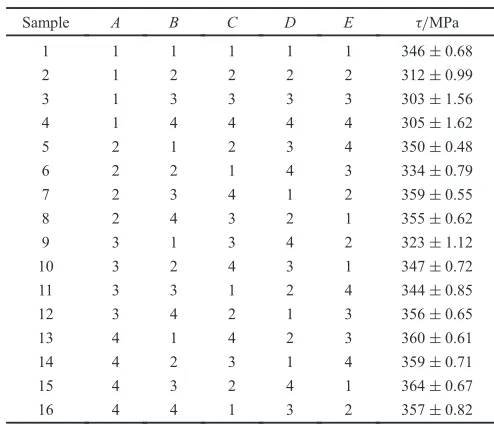
The orthogonal experiment were designed forfive factors and four levels of welding parameters of joint. The factors were concerned with controllable parameters such as brazing temperature (A), brazing time (B), diffusion temperature (C), holding time (D) and diffusion pressure (E), as shown in Table 1. The test value was joint shear strength (¸). The

results from the L16 (54) orthogonal array experiment are shown in Table 2.

The purpose of this orthogonal experiment is to improve the shear strength of joints, and therefore each value of factor (column) should select the maximal value (Table 3). The matrix K shows that thefirst element of the fourth level, the second element of the third level, the third element of the third level, the fourth element of the fourth level, and thefifth element of the third level. These were considered as a good test conditions, including brazing temperature (A) of 1045°C, brazing time (B) of 15 min, diffusion temperature (C) of 750°C, holding time (D) of 40 min and diffusion pressure (E) of 8 MPa. However, they should be tested, because the best combination of processes (A4B3C3D4E3) has not been found in the orthogonal experiment.

4. BP Neural Network Theories

Nofixed model can be solved in the material processing by using BP neural network. BP possesses a one-way commu-nication and feedback functions, three or more than three

Fig. 1 Processing diagram of vacuum hybrid welding.

Table 1 Levels and factors of the orthogonal experiment.

Level A/°C B/°C C/min D/MPa E/min

1 1015 650 0 2 5

2 1025 700 20 4 10

3 1030 750 40 6 15

4 1045 800 60 8 20

Table 2 Schedule of orthogonal experiment.

Sample A B C D E ¸/MPa

1 1 1 1 1 1 346«0.68

2 1 2 2 2 2 312«0.99

3 1 3 3 3 3 303«1.56

4 1 4 4 4 4 305«1.62

5 2 1 2 3 4 350«0.48

6 2 2 1 4 3 334«0.79

7 2 3 4 1 2 359«0.55

8 2 4 3 2 1 355«0.62

9 3 1 3 4 2 323«1.12

10 3 2 4 3 1 347«0.72

11 3 3 1 2 4 344«0.85

12 3 4 2 1 3 356«0.65

13 4 1 4 2 3 360«0.61

14 4 2 3 1 4 359«0.71

15 4 3 2 4 1 364«0.67

16 4 4 1 3 2 357«0.82

Table 3 Analysis of orthogonal experiment.

Range A B C D E

K

layers of neural network. It consists of input, hidden, and output layers. Weights and thresholds connect the upper and lower layers, and there is no connection between each layer of neurons. A three-layer BP network can be approximately close to any non-linear mapping modeling in theory. BP is composed of forward and backward network. In the forward propagation stage, each layer of neurons state affects only the next layer of neurons. If the output layer can not get the desired values, it will turn to the back propagation phase of error. In fact, the fast speed and high precision method10)can be found to adjust weights of network, which has the ability to learn from sets of examples and generalize this knowledge to new situations. In view of the statistical physics essence of ANN algorithm, error back-propagation BP neural network can solve nonlinear problems, it is expected to further improve the retrieval precision, based on the optimization of training samples and continue debugging of network type and parameters.11)_{Therefore, the BP network was developed in} Matlab software to establish the relationship between the vacuum hybrid welding and the shear strength of joints.

4.1 Design of BP network structure

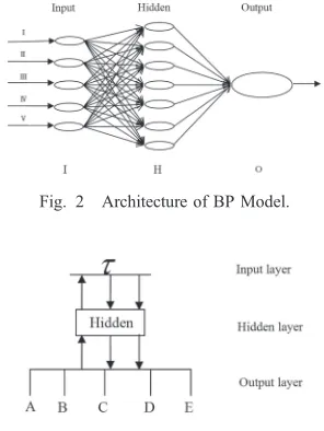
BP network is a kind of multilayer feed-forward neural network, whose transfer function of neurons is a S -Function,12)and the amount of continuous output is between 0 and 1.S-Function can achieve arbitrary non-linear mapping from input to output. The mapping relationship between high interactive process parameters and hardness of the YG8 cemented carbide and 42CrMo steel was established in vacuum hybrid brazing. According to the experimental conditions, a simple three-layer ANN model, which consists of input, hidden, and output layers, is selected for good performance as shown in Fig. 2. In the neural network terminology, the brazing temperature (A), brazing time (B), diffusion temperature (C), holding time (D) and diffusion pressure (E) were inputs while the shear strength (¸) of joints was output. The number of hidden layer nodes can be calculated by the following relationship:13)

n₁¼ ðmþnÞ12þa ð2Þ

where m is the number of output neurons; n is the number of input neurons; a is the constants from 1 to 10. Process parameters of BP network model are shown in Fig. 3.

The output g(x) produced by neuron i in layer L is described as follows:

gðxÞ ¼X

n

i

wixib¼XWb ð3Þ

where b is the offset or bias; wi is the weight vector, xi is input vector.

A neuron in the network produces its input by processing the net input via an activation (transfer) function which is usually non-linear. There are several types of activation functions used for BP. However, the tan-sigmoid transfer function is mostly used, which is assigned in hidden layer(s) for processing the inputs as the following relationship:

fx¼

1

1þex; 1< x <þ1 ð4Þ

and the differentiable function of (4) is as follows:

f0ðxÞ ¼fðxÞð1fðxÞÞ ð5Þ

4.2 Data normalization

The value of the activation functions of BP network is in the range of¹1 to+1, so the input data are correspondingly processed and transferred into the suitable scope. Then these data can better adapt to the output and reduce the weight adjustment. The normalized values (XA) for each raw in-put/ output dataset (Xi) was calculated as:14)

X0¼ ðXiXminÞ=ðXmaxXminÞ ð6Þ

where Xmax and Xmin are the maximum and the minimum values of raw data, respectively.

4.3 The training function selection

The proper function was selected for the proposed BP model. There are two training methods in Matlab (adding mode and batch mode). Adding mode is more suitable for the dynamic network, and batch mode needs to designate specify training function for the entire network. The mapping relationship between input and output can be achieved through training of input and output samples with learning and correction of weights and thresholds. LM (Lavenberg-Marquardt) algorithm,7)_{which comprises the Gauss-Newton} and the Steepest Descent method of algorithm, is a network training function that possesses local convergence and global features of gradient descent method. The relative errors obtained from this algorithm are smaller than that of any other algorithms.

4.4 BP network program

The BP model was designed by using Matlab toolbox. Experiments data were processed, trained and predicted by a simple three-layer BP model. The main procedures are as follows:

% The input and output of data:P=[+];T=[+];

% Normalization of experimental data: [pn,minp,maxp,tn, mint,maxt]=premnmx(p,t);

% BP neural network model: net=newff(minmax(pn), [N,1],{‘tansig’,‘tansig’},‘trainlm’);

% Network parameter settings: net.trainParam.show;

Fig. 2 Architecture of BP Model.

net.trainParam.Lr; net.trainParam.goal; net.trainParam.epoch;

% Load training results: TN=sim(net,pn);

% Network testing: L=[+];out=sim(net,pn);

5. Results and Analysis

The results can be obtained by using Matlab software with the training function through iterative computation on the computer. The input values P were transposed and the network model was established, because the values T of network output represented the row of the matrix. Mean-while, the parameters of network training were set, and Fig. 4 shows the training process.

Every training results are not the same, because the newff( ) function is random. And the Sim( ) function is used to simulate and verify the experiments in this work. The linear regression analysis of network is analyzed under the predictions and experiments. Figure 5 indicates that the output is better for tracking the actual value through the results of the statistical analysis, and the correlation coefficientRis 0.99898.

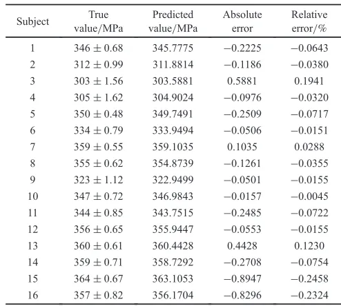
The outputs are compared with the true values to calculate the relative errors, as shown in Table 4.

Table 4 exhibits that relative errors of predicted values for test samples 3, 15 and 16 are ¹0.1941%, ¹0.2458% and ¹0.2324%, respectively, this is probably because the number of training data is relatively small, resulting in BP network being into the local minimum value points. From the experimental results in Table 4, it can be seen that the prediction results of BP neural network is quite accurate. By

comparing the recognition results and the experimental observations, it could be found that the relative errors are controlled in the range of«0.2%except for some individual samples, coinciding with the actual conditions.

Moreover, the mean square error (MSE) is calculated by the following relationship:

MSE¼ 1

NT

XT

m=1

XN

n¼1

½diðmÞ yiðmÞ2 ð7Þ

whereNis the number of outputs,Tis the number of training sets, di is the desired output, andyi is the network output. According eq. (7) the MSE for this ANN model is 0.052%. Consequently, the predicted values of the joints strength estimated by BP neural network are found to be in good agreement with the actual values from the experiments, and the ANN model could be used in predicting the joints strength of the YG8 cemented carbide and 42CrMo steel in vacuum hybrid welding.

6. BP Networks Prediction and Verification

The selected technology is consisted of 1024 kinds of process level combinations. As BP network is trained according to the above steps, it can be used to predict the shear strength of the joints under the process level combinations. The curve of the shear strength was drawn in more than 360 MPa, as shown in Fig. 6.

Figure 6 shows the undulating network forecasting curves, which reveals that different parameters combination signifi -cantly affect the shear strength of joints. No. 171 combina-tion parameters (A4B3C3D4E3) is the top of the BP network forecasting curves, and the shear strength is 363.8359 MPa, the welding condition of which includes brazing temper-ature (A) of 1045°C, brazing time (B) of 15 min, diffusion temperature (C) of 750°C, holding time (D) of 40 min and diffusion pressure (E) of 8 MPa. The process combination was preliminarily established for the best parameter

combi-Fig. 4 Network trainingfigure.

Fig. 5 Linear regression results of prediction set.

Table 4 Comparison of true values and predicted values on shear strength by BP ANN.

Subject True value/MPa

Predicted value/MPa

Absolute error

Relative error/%

1 346«0.68 345.7775 ¹0.2225 ¹0.0643 2 312«0.99 311.8814 ¹0.1186 ¹0.0380

3 303«1.56 303.5881 0.5881 0.1941

4 305«1.62 304.9024 ¹0.0976 ¹0.0320 5 350«0.48 349.7491 ¹0.2509 ¹0.0717 6 334«0.79 333.9494 ¹0.0506 ¹0.0151

7 359«0.55 359.1035 0.1035 0.0288

8 355«0.62 354.8739 ¹0.1261 ¹0.0355 9 323«1.12 322.9499 ¹0.0501 ¹0.0155 10 347«0.72 346.9843 ¹0.0157 ¹0.0045 11 344«0.85 343.7515 ¹0.2485 ¹0.0722 12 356«0.65 355.9447 ¹0.0553 ¹0.0155

13 360«0.61 360.4428 0.4428 0.1230

nation in the orthogonal experiment, which indicated a certain similarity between the BP networks predicted values and the orthogonal experiment results. However, the BP network easily fell into the local minimum value points, so four global optimal values were selected for the analysis. The relatively maximum points are the 118th group (A4B3C4D4E3), 126th group (A4B3C3D4E2), 154th group (A4B3C2D4E3), 176th group (A4B3C2D4E4), respectively, and the predicted values of the corresponding output are 363.7213 MPa, 363.6647 MPa, 363.5234 MPa and 363.6518 MPa, respectively, as shown in Fig. 6. These data are less than those of the 171st process combination. Therefore, the shear strength of the joint can be characterized by BP neural network.

The optimum process parameters predicted by BP was verified and tested. Shear strength is 364 MPa under the process parameters with relative error about 0.1%, by contrasts with the predicted value. Thus, BP can effectively reflect the feasibility of the non-linear relationship between the shear strength of joint and the process parameters.

7. Analysis of Characteristics of Hybrid Welding Joint

7.1 Microstructure and composition analysis of joints

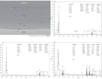
Figure 7 plots the EDS profile in different areas for typical hybrid welding joint, and the ingredients of features of region A,B,C,Dwere listed in Table 5. This observation shows that the best welding joint was achieved by vacuum hybrid brazing with good adhesion between the cemented carbide and nickel plating layer. There were no holes, no line defect and clear boundaries in the two kinds of materials, as shown in Fig. 7. As shown in Table 5, A district mainly consists of elements such as Fe, C, Ni, Cu; B district’s main components are Fe, C, Ni, Cu, Zn; C district is mainly composed of C, Ni, Cu, Zn; D district’s main ingredient are C, W, Co, Ni, Cu, Zn. Consequently, the copper element was main components in A, B and C areas. A small amount of Fe atoms were found in areas A and B, this maybe because a certain amount of Fe elements in 42CrMo steel diffused into the solder areas. However, the Fe atoms were not found in C area. Moreover, D area was Ni, Co and Cu, which existed as solid solution.

Fig. 6 The optimization combination forecast trend graph.

XRD was applied to the I, II and III areas after polishing of the welding joints (Fig. 8(a)), where the I area is close to the cemented carbide of the welding zone with forming a large tensile stresses, the II area locates in the interface between the cemented carbide and plated Ni layer, and the III area locates in the diffusion area between solder and Ni layer.

There are three areas that influence the mechanics properties of the cemented carbide. Figure 8(b) shows that YG8 components are WC, Co6W6C, Co3W and Co. Figure 8(c) shows that the main phase of II area is Ni matrix solution (FCC), WC and zinc or copper-zinc or nickel-zinc compounds. The III area consisted of nickel, cobalt, copper and zinc is shown in Fig. 8(d).

7.2 Micro-hardness analysis of the hybrid welding joints

The micro-hardness distribution of the hybrid welding joint is shown in Fig. 9. It is evident that the average value of the micro-hardness of the matrix after welding is 1476 HV, the micro-hardness of 42CrMo steel is 313 HV, and the minimum micro-hardness of brazing seam area is 187 HV.

7.3 Components analysis of welding joints either with or without Ni-plating

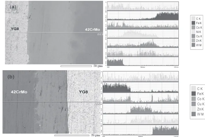
The width of the seam area of the joint with Ni-plating is about 70 µm (Fig. 10(a)), and the width of the seam area of joint without Ni-plating is 45 µm (Fig. 10(b)), which indicates that the width of seam area extends with the thickness of coatings increasing. In other words, the Ni atoms were diffused into the cemented carbide, and finally Ni and Co formed the infinite solid solution. Diffusion transition

Fig. 8 XRD analysis results of the typical joint (a) cross-section of joint

(b) -I, (c) -II, (d) -III. Fig. 9 Micro-hardness distribution of the typical hybrid welding joint.

Fig. 10 The EDS results of typical joint (a) and joint without Ni coating (b). Table 5 The EDS analysis from different region of the typical hybrid

welding joint.

Feature region

at.% C Fe Co Ni Cu Zn W

A 20.66 2.43 2.87 74.03

B 19.52 1.15 2.93 75.81 0.58

C 20.55 9.38 68.36 1.72

zone was achieved by mutual diffusion between YG8 and pure Ni. The solid solution possesses a good plasticity and high strength. Therefore, microstructure of welding joint was ideal. Thus, the toughness of the seam areas in the cemented carbide was improved.

8. Conclusion

This work showed the capability of BP network to predict the shear strength of joints by vacuum hybrid welding with the orthogonal experiment, and to optimize the results on the shear strength of the welding joint.

The optimal parameters of BP neural network were obtained at brazing temperature (A) of 1045°C, brazing time (B) of 15 min, diffusion temperature (C) of 750°C, holding time (D) of 40 min and diffusion pressure (E) of 8 MPa.

The complexity and limitations of the welding process can be effectively overcome by the BP neural network and the optimal process parameters can be provided for preparing the YG8 cemented carbide and 42CrMo steel in vacuum hybrid welding.

Acknowledgments

This work is supported by Shaanxi Industrial Science and Technology Research (2014K08-09) and the Scientific Research Program Funded by Yulin city (2012YLCXY112).

REFERENCES

1) Y. B. Hou, J. Y. Du and M. Wang: Neural network, (University of Electronic Science and Technology Press, Chengdu, 2007).

2) C. H. Dong: The Application of Matlab Neural Network, (National Defense Industry Press, Beijing, 2007).

3) Z. L. Wang, Z. X. Wang and X. Zhang: J. Chong Qing Jiao Tong Univ. (Natural Sci. Ed.)10(2010) 832­836.

4) Y. Z. Sun, W. D. Zhao, Y. L. Qi, Y. F. Han, Y. T. Shao and X. Ma: Rare Met. Mater. Eng.40(2011) 220­224.

5) Y. Y. Zong, D. B. Shan, M. Xu and Y. Lv:J. Mater. Process. Tech.209 (2009) 1988­1994.

6) Z. C. Sun, H. Yang and Z. Tang:Computational. Comp. Mater. Sci.50 (2010) 308­318.

7) K. L. Zhou and Y. H. Kang: Neural Network Model and MATLAB Simulation Program Design, (Tsinghua University press, Beijing, 2005).

8) D. N. Zou, H. B. Wang, Z. Y. Chen, Y. Han and J. H. Yu: Ordnance Mater. Sci. Eng.6(2011) 14­18.

9) W. C. Sun and C. Y. Miao: The brazing/diffusion vacuum hybrid welding method of cemented carbide and alloy steel. CN Patent. CN102922154B, published 30 July 2014.

10) Y. Shi, L. Q. Han and X. Q. Lian: Analysis and examples of the design method of neural network, (University of Posts and Telecommunica-tions press, Beijing, 2009).

11) L. Guan, Y. Liu and X. H. Zhang: Trans. Atmospheric Sci.33(2010) 341­346.

12) L. Guo, S. H. Wang and Q. M. Zhang: Appl. Laser12(2010) 479­482. 13) Y. Sun, W. D. Zeng and Y. Zhao: Rare Met. Mater. Eng.40(2011)

1951­1955.