Macroeconomic Effects of a Low Carbon Electricity Transition in Kenya and Ghana: An Exploratory Dynamic General Equilibrium Analysis

(1)

Munich Personal RePEc Archive

Macroeconomic Effects of a Low-Carbon

Electricity Transition in Kenya and

Ghana: An Exploratory Dynamic

General Equilibrium Analysis

Willenbockel, Dirk

Institute of Development Studies

March 2017

Online at

https://mpra.ub.uni-muenchen.de/78070/

(2)

Macroeconomic Effects of a Low-Carbon Electricity Transition in Kenya

and Ghana: An Exploratory Dynamic General Equilibrium Analysis

Dirk Willenbockel

Institute of Development Studies at the University of Sussex

in collaboration with

Helen H. Osiolo

Kenya Institute for Public Policy Research and Analysis

S. Bawakyillenuo

Institute of Statistical, Social and Economic Research, University of Ghana

February 2017

(3)

1

Abbreviations and Acronyms

AGRODEP African Growth & Development Modeling Consortium

aka Also known as

BaU Business as usual

bcf Billion cubic feet

CES Constant elasticity of substitution

CGE Computable general equilibrium

CPI Consumer price index

e.g. Exempli gratia (for example)

EnCG Energy Commission of Ghana

EPSRC Engineering and Physical Sciences Research Council

GDP Gross domestic product

GGDA Green growth diagnostics for Africa

GHG Greenhouse Gases

GLSS Ghana Living Standards Survey

GSS Ghana Statistical Service

GTAP Global Trade Analysis Project

GWh Gigawatt hours

GWS Gesellschaft für Wirtschaftliche Strukturforschung

ibid ibidem (in the same place)

i.e. id est

IFPRI International Food Policy Research Institute

IRENA International Renewable Energy Agency

ISSER Institute of Statistical, Social and Economic Research, University of Ghana

KIHBS Kenya Integrated Household Budget Survey

KIPPRA Kenya Institute for Public Policy Research and Analysis

KLEM Kapital Labour Energy Materials

KNBS Kenya National Bureau of Statistics

(6)

4 LAPSSET Lamu-Port Southern Sudan-Ethiopia Transport Corridor

LCO Light crude oil

LCOE Levelised cost of electricity

LES Linear expenditure system

LNG Liquefied natural gas

MW Megawatt

p.a. per annum

PV Photovoltaic

R2 _{Coefficient of determination}

RAS Bi-proportional matrix balancing method

SAM Social accounting matrix

SREP Sustainable Renewable Energy Program

SUT Supply and use tables

TD Transmission and distribution

TFP Total factor productivity

UN DESA United Nations Department for Economic and Social Affairs

UNDP United Nations Development Program

UNU-WIDER United Nations University - World Institute for Development Economics Research

USc United States cents

USD United States Dollars

(7)

5

1. Introduction

This study provides a forward-looking simulation analysis of economy-wide and distributional

implications associated with alternative pathways for the development of the electricity sector

in Ghana and Kenya. It is part of a wider research project that seeks to identify the binding

constraints to economically viable investments in renewable energy and to analyse the political

feasibility of a transition to a sustainable low carbon energy path in the two countries.

From an economic perspective, significant shifts in the power mix of an economy as well as

policy measures to induce or support such shifts are bound to affect the structure of domestic

prices across the whole economy with repercussions for the growth prospects of different

production sectors and for the real income growth paths of different socio-economics groups.

Understanding these economy-wide repercussions is crucial for a study concerned with the

obstacles to - and political feasibility of - adopting a low-carbon growth strategy. The analysis

requires the adoption of a multi-sectoral general equilibrium approach that allows to capture

the input-output linkages between the electricity sector and the rest of the economy as well as

the linkages between production activity, household income and expenditure and government

policy.

Thus, the present study develops purpose-built dynamic computable general equilibrium

(CGE) models for Ghana and Kenya with a detailed country-specific representation of the

power sector to simulate the prospective medium-run growth and distributional implications

associated with a shift towards a higher share of renewables in the power mix up to 2025.

The following section explains the methodological approach and describes the key features of

the CGE models in a non-technical manner. Each model is calibrated to a social accounting

matrix (SAM) which reflects the observed input-output structure of production, the commodity

composition of demand and the pattern of income distribution for the country at a disaggregated

level at the start of the simulation horizon. Section 3 spells out the data sources for the

construction of the social accounting matrices and outlines the model calibration process.

Sections 4 and 5 present the results of the dynamic simulation analysis for Kenya and Ghana

respectively. In each case, we first develop a stylised baseline scenario that simulates the

evolution of the economy under current power sector expansion plans up to 2025 and then

contrast these baselines with alternative lower carbon energy scenarios. Furthermore, the

sensitivity of results to alternative projections for world market fossil fuel prices is explored.

(8)

6

2. The Analytic Framework

2.1. Rationale for the Adoption of a CGE Approach

Computable general equilibrium (CGE) models – aka applied general equilibrium models – are

widely used tools in energy and climate mitigation policy analysis. Applications range from

short-run impact assessments of shocks to the energy system for particular countries to global

long-run energy system scenario studies with a time horizon of multiple decades.1

The prime appeal of – and need for - adopting a general equilibrium approach to energy policy

and energy-related environmental policy analysis arises from the fact that energy is an input to virtually every economic activity. Hence, changes in the energy sector ‘will ripple through multiple markets, with far larger consequences than energy’s small share of national income might suggest’ (Sue Wing, 2009). The unique advantage of the CGE approach over partial equilibrium approaches is its ability to incorporate these ‘ripple effects’ in a systematic manner.

In contrast to partial equilibrium approaches, CGE models consider all sectors in an economy

simultaneously and take consistent account of economy-wide resource constraints,

intersectoral intermediate input-output linkages and interactions between markets for goods

and services on the one hand and primary factor markets including labour markets on the other.

CGE models simulate the full circular flow of income in an economy from (i) income

generation through productive activity, to (ii) the primary distribution of that income to

workers, owners of productive capital, and recipients of the proceeds from land and other

natural resource endowments, to (iii) the redistribution of that income through taxes and

transfers, and to (iv) the use of that income for consumption and investment (Pueyo et al, 2015).

2.2. Specification of the Dynamic CGE Models for Kenya and Ghana

In terms of theoretical pedigree, the CGE models for Kenya and Ghana employed in this study

can be characterized as modified dynamic extensions of standard comparative-static

single-country CGE models for developing countries in the tradition of Dervis, de Melo and Robinson

(9)

7 (1982), Robinson et al (1999) and Lofgren et al (2002). Models belonging to this class have

been widely used in applied development policy research. Apart from the incorporation of

capital accumulation, population growth, labor force growth and technical progress,2 the main

difference to the standard model is a more sophisticated specification of the electricity sector

as detailed below.

2.2.1. Domestic Production and Input Demand

Domestic producers in the model are price takers in output and input markets and maximize

intra-temporal profits subject to technology constraints. The technologies for the

transformation of inputs into real outputs are described by sectoral constant-returns-to scale

production functions. In line with common practice in energy-focused top-down CGE models,3

technology specifications belonging to the generic class of KLEM (Capital (K), Labour,

Energy, Materials) production functions are employed to capture substitution possibilities

among energy and-non-energy inputs and among different energy sources. In technical terms,

the sectoral KLEM production functions take the form of nested multi-level functions with a

(positive or zero) constant elasticity of substitution (CES) among inputs grouped together

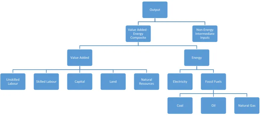
within the same nest. Figure 1 provides a schematic representation of the substitution hierarchy

between different inputs in production in the model.

In each sector, the production of a given output quantity requires non-energy inputs and a

composite value-added/energy composite in fixed proportions. The value added/energy

composite requires energy and primary factors (i.e. skilled and unskilled labour, capital, land

and natural resources) in variable proportions. Thus, when the composite price index of energy

rises relative to primary factor prices, energy inputs are replaced to some extent by additional

inputs of primary factors. In other words, the model generates a shift towards less

energy-intensive modes of production in response to an increase in energy prices. Required energy

inputs are composed of electricity purchases from the electricity sector in the model and direct

use of fossil fuels. The model allows substitution of these primary fossil energy carriers for

electricity in sectors where the input-output matrices of the GTAP database record intermediate

2_{See e.g. Arndt, Robinson and Willenbockel (2011) and Robinson, Willenbockel and Strzepek (2012) for earlier} recursive-dynamic extensions of the standard model.

(10)

8 purchases of fossil fuels. At the bottom of the input substitution hierarchy, the sectoral

production functions allow for imperfect substitutability between coal, refined oil and natural

[image:10.595.72.506.251.451.2]

gas.

Figure 1: Production Function Nesting Structure

2.2.2. Electricity Supply

In standard energy-focused top-down CGE models, electricity generation and distribution is

typically treated as a single production activity. In these models a transition towards a higher

share of hydro, solar or wind in the power mix is represented in a highly stylized abstract form

as a substitution of fossil fuel inputs by physical capital under the assumption of a continuous

space of available technologies. The lack of explicit detail with regard to the characterization

of current and future technology options entails the danger that in the case of simulation

scenarios involving large departures from the initial benchmark equilibrium may violate

fundamental physical restrictions such as the conservation of matter and energy (Böhringer and

Rutherford, 2008) or exceed other technical feasibility limits (McFarland, Reilly and Herzog,

2004; Hourcade et al, 2006; Bibas and Mejean, 2012). Moreover, the lack of technological

explicitness limits the ability of top-down models to incorporate detailed information on cost

differentials among alternative energy technologies from engineering cost studies and to

Output

Value Added -Energy Composite

Value Added

Unskilled

Labour Skilled Labour Capital Land

Natural Resources

Energy

Electricity Fossil Fuels

Coal Oil Natural Gas

(11)

9 simulate technology-specific policy measures in a fully persuasive manner (Hourcade et al,

2006). In response to these limitations of conventional top-down CGE models, various approaches to the incorporation of detailed ‘bottom up’ information on energy technology options into a CGE modelling framework have emerged.4

The present study adopts a similar hybrid top-down bottom-up approach by treating

decomposing electricity generation according to power source and by treating electricity

transmission / distribution as a separate activity. This approach enables us to incorporate extant

information on levelised cost of electricity (LCOE) differentials by power source into the

simulation analysis and to consider exogenous policy-driven changes in the power mix that are

not necessarily driven by changes in relative market prices. The system-wide supply price of

electricity in the models is effectively determined as weighted average of the activity-specific

supply prices across the power activities. The operational aspects of the power sector

decomposition are outlined in section 3 below.

2.2.3. Primary Factor Supply

The model distinguishes skilled and unskilled labour. The dynamic labour supply paths are

exogenous and both types of labour are intersectorally mobile. The supply of agricultural land

and natural resource endowments (forests, minerals, and in the case of Ghana crude oil and

natural gas) is imperfectly elastic, i.e. the supply of these primary factors varies endogenously

in response to changes in the corresponding factor price. The productive capital stock in each

sector a evolves according to the dynamic accumulation equation K(a,t+1) = I(a,t) + (1 –δ(a))K(a,t),

where K denotes the installed real capital stock, I(a,t) is real gross investment flowing to sector a in period t and δ is the rate of physical capital depreciation. Sectoral gross investment is a positive function of a sector’s rate of return to capital relative to the economy-wide average

return to capital, i.e. the sectoral allocation of aggregate real investment is determined by return

(12)

10 differentials. Once installed, capital is sector-specific (i.e. immobile across sectors) while new

capital is intersectorally mobile.

2.2.4. Final Domestic Demand

Consumer behavior is derived from intra-temporal utility maximizing behavior subject to

within-period budget constraints. Utility functions take the Stone-Geary form, yielding a

Linear Expenditure System (LES) demand specification. The commodity composition of

investment and government demand is kept constant according to the observed shares in the

benchmark SAM while the total volumes of government and investment demand grow in line

with aggregate income and are determined by the macro closure rules detailed below.

2.2.5. International Trade

In all traded commodity groups, imports and goods of domestic origin are treated as imperfect

substitutes in both final and intermediate demand. Agents’ optimizing behaviour entails that

the expenditure-minimizing equilibrium ratio of imports to domestic goods in any traded

commodity group varies endogenously with the corresponding relative price of imports to

domestically produced output in that commodity group.

On the supply side, the model takes account of product differentiation between exports to the

rest of the world and production for the domestic market in all exporting sectors. The

technologies for conversion of output into exports are described by sectoral

constant-elasticity-of- transformation (CET) functions. This entails that the profit-maximizing equilibrium ratio

of exports to domestic goods in any exporting sector is determined by the price relation between

export and home market sales.

Both Kenya and Ghana are treated as small open economies – i.e. changes in their export supply

and import demand quantity have no influence on the structure of world market prices.

2.2.6. Equilibrium Conditions and Macro Closure

The prices for goods, services and primary factors are flexible and adjust in order to satisfy the

(13)

11 account balance follow an exogenous time path. This time path is kept fixed across the

simulation scenarios considered in subsequent sections in order to enable meaningful welfare

comparisons across the scenarios. This external sector closure entails that the real exchange

rate adjusts endogenous to maintain external balance-of-payments equilibrium. A standard

balanced macroeconomic closure rule (Lofgren et al, 2002) is adopted, according to which the

shares of government demand, investment demand and hence private household consumption

demand in total absorption remain invariant. Under this macro closure, household and

government saving rates adjust residually to establish the macroeconomic saving-investment

(14)

12

3. Data Sources and Model Calibration

3.1. The Social Accounting Matrices for Kenya and Ghana: Overview

Each model is calibrated to a SAM which reflects the input-output structure of production, the

commodity composition of demand and the pattern of income distribution for the country at a

disaggregated level at the start of the simulation horizon. Starting point for the construction of

the model-conformable SAMs are the input-output matrices for Kenya and Ghana contained in

the GTAP database version 9 (Aguiar, Narayanan and McDougall, 2016). This data set

provides a detailed and internally consistent representation the global economy-wide structure

of production, demand and international trade at a regionally and sectorally disaggregated

level. GTAP 9a – the latest available version of the database - combines detailed bilateral trade

and protection data reflecting economic linkages among 140 world regions with individual

regional input-output data, which account for intersectoral linkages among 57 production

sectors for the benchmark year 2011.5

The GTAP database treats electricity generation, transmission and distribution as a single

aggregate activity and the data on household income and household consumer expenditure are

for a single aggregate household. For the purposes of the present study, both the electricity

activity and the household sector are disaggregated as detailed below.

3.2. Disaggregation of the Electricity Sector

The decomposition of the power activity for each country essentially involves (i) splitting the

single electricity activity column vector of the original GTAP input-output matrix (which

contains the annual input cost by input type for the benchmark year) into several new columns

for the different electricity sub-sectors distinguished in the CGE model, and (ii) distributing

(15)

13 the cost figures of the original aggregate electricity cost vectors horizontally across the new

columns in line with available information about the cost composition in the electricity

sub-sectors and in such a way that the original cost totals by input type are preserved. This is a

non-trivial problem. The common procedure employed in the construction of databases for

energy-focused hybrid top-down bottom-up CGE models is to start with an informed initial estimate

for the entries in the new sub-industry column vectors and then apply a numerical matrix

balancing method to enforce the target sub-matrix totals.6

Peters (2016) constructs a satellite database for GTAP9 which disaggregates the GTAP

electricity activity for all regions in the database along these lines. However, the regional

coverage of LCOE estimates used in the construction of the Peters database is incomplete, with

country-specific estimates for Africa being notable by their virtual absence.7 In cases, where

the discrepancies between the row totals implied by the initial guesses in the absence of

country-specific data and the target GTAP row totals is large, the application of the mechanical

matrix balancing algorithm can generate seriously misleading results. The case of Kenya –

flagged up explicitly by Peters (2016:231, n12) as a problematic case – illustrates the point: In

the benchmark year 2011 Kenya generates electricity primarily from hydro, thermal (i.e. fossil

fuel) and geothermal sources8. Geothermal is not identified as a separate technology in the

Peters database, but would in principle be covered one-to-one by the residual “Other” category

in that data base. Yet, attributing the reported cost figures in this category to geothermal would

lead to seriously misleading results.9

Therefore, the decomposition of the electricity sectors for the present study uses additional

country-specific data and information from other studies. For Kenya, the electricity activity is

disaggregated into transmission and distribution (TD), hydro, geothermal, thermal and wind.

First, the cost totals for the sub-activities are determined: The TD share is based on Peters

(2016) while the total generation share is distributed across the four generation activities by

combining the 2011 electricity generation data in GWh reported in Republic of Kenya (2014:

6_{See Peters and Hertel (2016a,b) for a detailed discussion of comparison of existing matrix balancing algorithms} used in this context and further references to the related technical literature.

7_{See Peters (2016: Appendix C). As Peters (2016:216) puts it,}“(i)_{ncreasing the LCOE coverage is a major} opportunity for subsequent versions”.

8_{See Table 5 below.}

(16)

14 Table 33)10 with the LCOE cost differential estimates for Kenya (Table 1) reported in Pueyo

et al (2016). Fossil fuel input are entirely allocated to the thermal electricity activity while

initial estimates for the allocation of other inputs are informed by the cost shares for the

different generation technologies in the Peters (2016) database and - for geothermal – on cost

share data from Sue Wing (2008) and Lehr et al (2011).11 Finally, to establish full consistency

of the cost entries with the GTAP cost totals by input type and the target electricity sub-activity

column sums, a standard bi-proportional RAS matrix balancing algorithm is employed.

The electricity sector decomposition for Ghana splits the sector into TD, hydro and thermal

and follows the same procedural approach. The required physical data on power generation by

technology for the benchmark year 2011 are drawn from EnCG (2016).

The resulting synthetic cost vectors capture the salient stylized facts with regard to input

intensities of the different electricity generation technologies, namely that hydro, geothermal

and wind are very capital-intensive and have moderate intermediate input requirements,

geothermal is particularly skill-intensive and fossil fuel costs are the dominant cost factor in

thermal generation (and more so in high-fossil-price periods such as in the benchmark year

2011).

Table 1 Levelised Cost of Electricity by Technology and Country

Ghana Kenya

Hydro 6.8 - 11.2 7.4 - 10.9

Wind 12.6 - 19.5 7.7 - 10.3

Geothermal Not applicable 4.7 - 7.5

Solar PV 16.0 - 26.9 9.9 - 14.8

Thermal - Oil 19.0 26.0 - 42.0

Thermal - Gas 13.0 13.3

Source: Pueyo et al (2016).

10_{See Table 5 below.}

(17)

15

3.3. Disaggregation of the Household Accounts

The household disaggregation for Ghana distinguishes five household groups - labelled H1

(bottom quintile) to H5 (top quintile) - by household income quintile in the benchmark year.

The available data sources do not support a consistent rural-urban split. Information on the

distribution of factor income is drawn from the Ghana Living Standards Survey (GLSS 6)

(GSS, 2014: Section 10). To establish full consistency with the economy-wide functional

household income distribution by factor type given by the GTAP database while preserving

the GLSS factor income distribution by household quintile, a bi-proportional matrix balancing

algorithm is used. In the benchmark year households in the top quintile receive 45.6 percent of

total income while the share of the bottom quintile is 5.3 percent. For H1 to H4 the main income

source is low-skilled employment (including imputed labour income from self-employment),

whereas the dominant income source for H5 is skilled employment. Top quintile households

also receive the largest shares of total capital and natural resource rent income. The

decomposition of the aggregate household consumption vector by commodity group from the

GTAP database uses household expenditure shares by quintile derived from GLSS.

For Kenya, no recent representative household income and expenditure survey is available.

The last survey is the Kenya Integrated Household Budget Survey (KIHBS) 2005/06. As the

published KIHBS results provides insufficient detail on the income distribution by income

type, the household sector decomposition for Ghana draws upon the household disaggregation

generated by Kiringai et al (2007) for the KIPPRA-IFPRI SAM, which is based on an earlier

survey for 1997 and distinguishes urban and rural households by expenditure decile.

Employing such a dated source is obviously unsatisfactory. However, Gakuro and Mathenge

(2012:Table 2) show that there is remarkably little change between the 1997 and the 2005/06

expenditure distribution, except for a marked 5 percentage-point gain for the top urban decile

primarily at the expense of the ninth and eighth decile and to a lesser extent at the expense of

the bottom two deciles. Thus, across broader household aggregates the distribution is almost

stable between 1997 and 2005/06, e.g. the share of the top 5 rural deciles remains constant at

75 percent, while the share of the top 5 urban deciles rises modestly from 77 to 79 percent.12

12_{An inspection of the corresponding KIHBS and 1997 data in World Bank (2008) and in the UNU-WIDER} (2017) WIID database confirms this finding. It must be noted though that over this period the urban share of

(18)

16 Correspondingly, the Kenya SAM and model uses a coarse household disaggregation with four

household groups – labelled Rural Low, Rural High, Urban Low and Urban High – which

represent respectively the bottom and top 50% rural and urban households in the benchmark

year. In short, a more detailed household disaggregation is not supported by the available data

at this point in time.

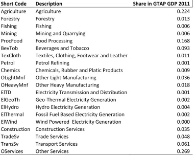
3.4. SAM Dimensions

The benchmark SAM for Kenya distinguishes 19 production activities (Table 1), 7 primary

production factors including 3 sector-specific natural resource factors (forest, fish and mineral

stocks) beside skilled and unskilled labour, capital, and agricultural land and 4 household

categories. The Ghana SAM for the benchmark year contains 18 production activities (Table

2), 8 primary factors including oil / gas resource stocks in addition to the same factors as in the

Kenya SAM, and 5 household groups. Both SAMs contain 18 commodity groups (Agriculture,

Forestry, Fishing, Crude Oil, Natural Gas, Other Mining, Beverages and Tobacco, Processed

Food, Textiles and Clothing including Footwear and Leather Goods, Refined Petrol, Chemicals

including Plastic and Rubber Goods, Other Light Manufacturing, Other Heavy Manufacturing,

Electricity, Construction Services, Trade Services, Other Services).

3.5. Model Calibration

The numerical calibration process involves the determination of the initial model parameters

in such a way that the equilibrium solution for the benchmark year exactly replicates the

benchmark SAM. The selection of values for the sectoral factor elasticities of substitution, the

elasticities of substitution between imports and domestically produced output by commodity

group, and the target income elasticities of household demand is informed by available

econometric evidence from secondary sources and uses estimates provided by the GTAP

behavioral parameter database (Hertel and van der Mensbrugghe, 2016). The region-specific

income elasticity estimates reported in that source for a representative single aggregated

household are further differentiated across the lower and higher income households in the

model, e.g. for necessary goods such as food products with an observed higher budget share in

low-income households, the initial elasticities are raised vis-à-vis the central GTAP values and

(19)

17 Given the selection of these free parameters, the various share parameters of the models –

including the effective initial direct and indirect model tax rates – are then entirely identified

by the benchmark SAMs. Several of the model parameters, such as the factor productivity

parameters governing the rate of autonomous technical progress are time-variant in the

dynamic simulation analysis. The dynamic calibration of these time-variant parameters is

discussed in the context of the description of the dynamic baseline construction process in

(20)

[image:20.595.76.461.96.401.2]

18 Table 1: Kenya Model Production Sectors

Short Code Description Share in GTAP GDP 2011

Agriculture Agriculture 0.224

Forestry Forestry 0.013

Fishing Fishing 0.006

Mining Mining and Quarrying 0.006

ProcFood Food Processing 0.168

BevTob Beverages and Tobacco 0.093

TexCloth Textiles, Clothing, Footwear and Leather 0.011

Petrol Petrol Refining 0.001

Chemics Chemicals, Rubber and Platic Products 0.009 OLightMnf Other Light Manufacturing 0.036 OHeavyMnf Other Heavy Manufacturing 0.018 ElTD Electricity Transmission and Distribution 0.001 ElGeoTh Geo-Thermal Electricity Generation 0.002 ElHydro Hydro Electricity Generation 0.004 ElThermal Fossil Fuel Based Electricity Generation 0.002 ElWind Wind Powered Electricity Generation 0.000 Construction Construction Services 0.035

TradeSv Trade Services 0.048

TransSv Transport Services 0.061

OServices Other Services 0.269

Table 2: Ghana Model Production Sectors

Short Code Description Share in GTAP GDP 2011

Agriculture Agriculture 0.236

Forestry Forestry 0.007

Fishing Fishing 0.018

CrudeOil Crude Oil and Natural Gas 0.063

Mining Mining and Quarrying 0.008

ProcFood Food Processing 0.042

BevTob Beverages and Tobacco 0.010

TexCloth Textiles, Clothing, Footwear and Leather 0.012

Petrol Petrol Refining 0.001

Chemics Chemicals, Rubber and Platic Products 0.008 OLightMnf Other Light Manufacturing 0.018 OHeavyMnf Other Heavy Manufacturing 0.031 ElTD Electricity Transmission and Distribution 0.001 ElHydro Hydro Electricity Generation 0.008 ElThermal Fossil Fuel Based Electricity Generation 0.000 Construction Construction Services 0.138

TradeSv Trade Services 0.054

TransSv Transport Services 0.105

[image:20.595.77.452.466.757.2]

(21)

19

4. Dynamic Scenario Analysis: Kenya

4.1. Overview

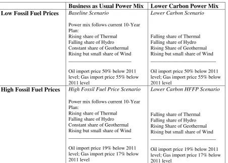
The simulation analysis for Kenya considers four dynamic scenarios up to 2025 that differ with

respect to (i) the evolution of the power mix in on-grid electricity generation and (ii) the

evolution of world market fossil fuel prices. Table 3 provides a concise outline of the alternative

scenario assumptions along these two dimensions.

The specification of the lower carbon scenarios is motivated by the results of the comparative

LCOE analysis by Pueyo et al (2016, 2017) which indicates a clear cost advantage of

geothermal over all other electricity generation technologies and by the presence of a

considerable potential for the further expansion of geothermal capacity in the country. The

consideration of alternative conceivable time paths for the evolution of international fossil fuel

prices is motivated by the strong sensitivity of the cost differences between thermal and

[image:21.595.76.529.425.748.2]

renewables to fossil price projections.

Table 3: Schematic Outline of Scenarios for Kenya

Business as Usual Power Mix Lower Carbon Power Mix Low Fossil Fuel Prices Baseline Scenario

Power mix follows current 10-Year Plan:

Rising share of Thermal Falling share of Hydro Constant share of Geothermal Rising but small share of Wind _________________________

Oil import price 50% below 2011 level; Gas import price 55% below 2011 level

Lower Carbon Scenario

Falling share of Thermal Falling share of Hydro Rising Share of Geothermal Rising but small share of Wind __________________________

High Fossil Fuel Prices High Fossil Fuel Price Scenario

Power mix follows current 10-Year Plan:

Rising share of Thermal Falling share of Hydro Constant share of Geothermal Rising but small share of Wind _________________________

Lower Carbon HFFP Scenario

Falling share of Thermal Falling share of Hydro Rising Share of Geothermal Rising but small share of Wind __________________________

(22)

20

4.2. Baseline Scenario

The dynamic baseline scenario provides a projection of the evolution of Kenya’s economy up

to 2025 under the assumptions that international oil and gas prices remain at low 2015/16 levels

and that the evolution of the electricity generation capacity from hydro, geothermal and wind

follows Kenya’s 10 Year Power Sector Expansion Plan 2014-2024 (Republic of Kenya, 2014) under the Plan’s moderate load growth scenario.

The construction of the baseline scenario starts from the 2011 benchmark SAM outlined in

section 3. For the period up to 2015, the forward projection takes account of the most recent

available data observations, while the projections from 2016 to 2025 draw upon expert

forecasts for the determination of the main model-exogenous drivers of economic growth

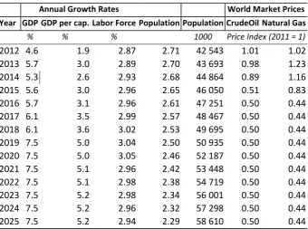
(Table 4). 13

4.2.1. Population and Labour Force Growth

Population and labour force growth is based on the UN DESA (2015) medium-variant

projections commonly used in contemporary long-run scenario studies. According to these

projections, the total population of Kenya rises from 42.5 million in 2012 to 58.6 million in

2025. As shown, the scenario takes into account that over this period the annual growth rate of

the working-age population – and thus the labour force growth rate in the model under the

assumption of a constant participation rate - remains considerably higher than the population

growth rate.

4.2.2. Total Factor Productivity and GDP Growth

The second exogenous driver of economic growth in the model is the economy-wide total

factor productivity (TFP) growth rate, which reflects the speed of autonomous technical

progress. In the development of the baseline scenario, the time path for the annual TFP growth

rate is determined indirectly by imposing a target growth path for Kenya’s real gross domestic

product (GDP) (see Table 4) and by calibrating the TFP parameter of the model dynamically

(23)

21 to match this target growth path. Technically, to obtain the TFP growth path the model is first

simulated in a dynamic calibration mode in which GDP is exogenized while the TFP parameter

is treated as an endogenous variable. When the model is then simulated in normal mode, with

GDP as an endogenous variable and exogenous imposition of the TFP growth path obtained in

the dynamic calibration run, the model solution exactly replicates the target GDP growth path.

The GDP baseline scenario growth rates up to 2015 are the reported actual national accounts

figure and the projections up to 2018 are taken from KIPPRA (2016). The assumed constant

growth rate of 7.5 percent per annum beyond 2018 is an optimistic compromise between the annual growth rate target of 10 percent envisaged in Kenya’s aspirational Vision 2030 development plan (Republic of Kenya, 2007) for the same period and the growth rates projected

by the CGE model under the assumption that TFP grows at a moderate pace that is more in line with the country’s actual observed growth performance over recent years: The average annual TFP growth rate for the period 2011-2015 that is required in the model to replicate Kenya’s

actual GDP growth reported in Table 4 is 0.8 percent14 and the corresponding rate for the period

2016 to 2018 is 2.8 percent. To reach the assumed 7.5 percent GDP growth rate beyond 2018,

the average annual TFP growth rate needs to rise further to reach 3.3 percent. Thus, the baseline

scenario implies a strong acceleration in the growth rate of technical progress, yet the TFP

growth rate figures are not entirely implausible, provided a significant portion of the measures

to modernize the economy envisaged in the Kenya Vision 2030 are actually implemented over

the time horizon considered here. However, GDP growth rates on the order of 10 percent per

annum would require TFP growth rates well above 5 percent. Assuming a sustained

productivity acceleration of such an order would seem to be unrealistic, given Kenya’s actual

growth performance under the Vision 2030 plan so far.15

14_{This CGE-model-determined figure matches closely with the corresponding growth-accounting-based estimate} of 0.8 percent TFP for Kenya in 2015 and average annual TFP growth of 0.6 percent over the period 2011 to 2015 presented in The Conference Board (2016).

15_{As shown in Republic of Kenya (2013: Table 2.1), in every single year of the first five-year implementation} phase (2008/9 to 2012/13) Kenya missed the Vision 2030 GDP growth targets by a wide margin (i.e. by 4.0 to 4.6 percentage points). Despite a downward revision of the target rates for 2013 to 2015 (ibid: Table 2.2), Kenya’s

(24)

[image:24.595.73.414.92.345.2]

22 Table 4: Key Features of Dynamic Baseline Scenario - Kenya

Annual Growth Rates World Market Prices

Year GDP GDP per cap. Labor Force Population Population CrudeOil Natural Gas

% % % 1000 Price Index (2011 = 1) 2012 4.6 1.9 2.87 2.71 42 543 1.01 1.02 2013 5.7 3.0 2.89 2.70 43 693 0.98 1.23 2014 5.3 2.6 2.93 2.68 44 864 0.89 1.16 2015 5.6 3.0 2.96 2.65 46 050 0.51 0.83 2016 5.7 3.1 2.96 2.61 47 251 0.50 0.44 2017 6.1 3.5 2.99 2.57 48 467 0.50 0.44 2018 6.1 3.6 3.02 2.53 49 695 0.50 0.44 2019 7.5 5.0 3.04 2.50 50 935 0.50 0.44 2020 7.5 5.0 3.05 2.46 52 187 0.50 0.44 2021 7.5 5.1 2.96 2.42 53 448 0.50 0.44 2022 7.5 5.1 2.98 2.38 54 719 0.50 0.44 2023 7.5 5.2 2.98 2.34 56 001 0.50 0.44 2024 7.5 5.2 2.96 2.32 57 298 0.50 0.44 2025 7.5 5.2 2.94 2.29 58 610 0.50 0.44 Sources: GDP growth: 2012, KNBS (2016); 2013-18 KIPPRA (2016); Population and labour force growth: UN DESA (2015), medium-variant projections.

4.2.3. Electricity Sector

The assumed evolution of the power mix in the baseline scenario draws upon Kenya’s 10 Year Power Sector Expansion Plan 2014-2024 (Republic of Kenya, 2014) while taking into account

that under the assumed baseline economic growth path, the electricity demand growth over the

simulation horizon endogenously generated by the CGE model is significantly lower than in

the 10-Year Plan: This plan considers a high growth scenario with a ‘fast-tracked’

implementation of a range of energy-intensive Vision 2030 flagship investment projects16 and a ‘moderate load growth scenario’with a ‘deferred’ implementation of these flagship projects.

The high growth scenario assumes that GDP growth reaches 10.1 percent p.a. by 2018 and

accelerates further to 12 percent p.a. by 2024. Effective electricity demand is projected to grow

at average annual rate of 17.4 percent between 2015 and 2024 to reach 56,447 GWh by 2024

(25)

23 (Republic of Kenya, 2014: Table 28) Based on least cost power expansion simulations17, this

scenario proposes a strong expansion in hydro capacity (+74 percent relative to 2013) and

massive expansions in geothermal (+1,200 percent), thermal (~ +2,400 percent) and wind (~

+18,600 percent from a tiny base) by 2024 to satisfy this demand growth (Republic of Kenya,

2014: Table 25). The projected domestic generation shares in 2024 under average hydrological

conditions in this scenario are 47.2 percent for geothermal, 42.5 percent for thermal, 9.5 percent

for hydro and 0.8 percent for wind. The scenario envisages that coal-fired power generation

starts in 2016 and then rapidly expands to reach a share of 17.4 percent in total generation by

2024. With respect to the plausibility and economic viability of this scenario, the Plan itself

states that

“under the fast-tracked scenario, there would be a huge power surplus if demand does not grow fast enough which could lead to stranded investments and/or high power tariffs. Additionally, the report reveals that high cost technologies such as the thermal power plants particularly those planned for commissioning in 2014 may be poorly dispatched in the medium to long term while base plants such as coal and LNG may end up being run at below optimal levels of less than 70%” (Republic of Kenya, 2014:5).

According to the latest KNBS (2016b) figures actual electricity generation in 2015 was some

30 percent below the corresponding 2015 projection under this scenario and the plans for the

construction of Kenya’s first coal-fired power plant in Lamu as well as related plans for the

exploitation of domestic coal resources detected in the Mui Basin are on hold.18 Thus, the 10-Year Plan’s high growth scenario provides no suitable basis for the development of a plausible baseline scenario for purposes of the present study.

The ‘moderate load growth’ scenario of the 10-Year plan assumes that annual GDP growth rises to 10 percent by 2020 and that the economy continues to grow at that rate up to 2024. The

aforementioned flagship investments are implemented slightly later than in the high growth

scenarios and the connection rate reaches 60 percent by 2024. Effective electricity demand is

projected to grow at average annual rate of 15.5 percent between 2015 and 2024 and reaches

38,413 GWh by 2024 (Republic of Kenya, 2014: Table 33). Hydro capacity is projected to

jump by 61 percent in 2019 relative to a constant 2014-2018 level with no further expansion

up to 2024, geothermal capacity expands by 288 percent between 2014 and 2024, thermal by

322 percent, and wind generation capacity expands by a factor of 24.5 relative to the small

2014 level (Republic of Kenya, 2014: Table 32). The projected domestic generation shares in

17_{These simulations are an update of the earlier 2013 Least Cost Power Sector Development Plan (Republic of} Kenya, 2013b).

(26)

24 2024 in this scenario are 48.2 percent for geothermal, 39.2 percent for thermal, 11.7 percent

for hydro and 0.8 percent for wind. Coal-fired power plants start operating from 2019 and reach

a share of 20.9 percent in total domestic electricity generation by 2024.

As discussed in section 4.2.2 above, our baseline scenario is an optimistic scenario but uses

lower GDP growth projections than the 10-Year Plan’s so-called ‘moderate load growth scenario’. Correspondingly, the electricity demand growth projected by the CGE model - which equates to an annualized average growth rate of 12.8 percent over the period 2015 to 2025 - is

significantly below the Plan’s average annual growth rate of 15.5 percent. In absolute terms,

this demand growth differential translates into a marked difference between the 2025

CGE-model-based baseline projection of 35,641 GWh (Table 5) for domestic supply and a one-year

forward projection of the Plan’s 2024 domestic supply, which amounts to nearly 44,000

GWh.19 It is noteworthy, that this difference is larger than the entire projected coal-based

generation for 2024 (7,965 GWh) according to the Plan. Thus, no coal-fired power-plants at all

are required in our baseline scenario.

Table 5: Domestic Electricity Generation by Type – Baseline Scenario

Electricity Generation (GWh)

Year Total Hydro Geothermal Thermal Wind

2011 7250 3427 1453 2352 18 2015 10675 3427 5333 1868 47 2020 22735 4466 11343 6829 97 2025 35641 4466 18331 12529 315

Shares (%)

2011 100.0 47.3 20.0 32.4 0.2 2015 100.0 32.1 50.0 17.5 0.4 2020 100.0 19.6 49.9 30.0 0.4 2025 100.0 12.5 51.4 35.2 0.9 Sources: All figures for 2011 and all GWh figures for Hydro, Geothermal and Wind: Republic of Kenya (2014: Tables 6 and 33). Domestic total generation figures are model- determined and Thermal shares beyond 2015 follow residually. Actual provisional 2015 figures in KNBS (2016b) released after the completion of the baseline construction: Total: 9456 GWh, Hydro: 3463 GWh (36.6%), Geothermal: 4521 GWh (47.8%), Thermal 1412 GWh (14.9%).

(27)

25 As shown in Table 5, the baseline scenario assumes that hydro, geothermal and wind generation

evolves in line with the moderate load growth scenario of the 10 Year Power Sector Expansion

Plan20 while thermal (gas- and oil-fired) generation fills the gap between total demand and

non-fossil-based supply. Correspondingly, the direction of the changes in the power mix over the

period 2015 to 2025 are broadly in line with the 10-Year Plan moderate scenario, in the sense

that (i) the hydro share drops markedly despite a substantial increase in absolute capacity, (ii)

the geothermal share remains roughly constant following the rapid increase over the period

2011 to 2015, which means that absolute geothermal generation grows strongly and

approximately in proportion to total electricity demand, (iii) the share of thermal rises strongly,

and (iv) the wind share roughly doubles but remains below one percent.

The main difference to the Plan scenario is that, due to the lower overall electricity demand

growth, the baseline 2025 thermal share is slightly lower (35.2 versus 39.2 percent) and greener

as it contains no coal-fired generation.

According to the moderate load growth scenario, the share of diesel within total non-coal

thermal generation, which was 100 percent in the benchmark year 2011, drops markedly to 58

percent in 2015 and further to 14 percent in 2024 as diesel-fired generation is replaced by

gas-fired generation. However, as the recent cancellation of the planned Dongu Kundu gas power

station project indicates21, such a shift appears unlikely to happen within the time horizon of

the present study. Thus the baseline scenario assumes that thermal generation continues to

remain entirely heavy-fuel-oil-fired. Nevertheless the cost disadvantage of thermal relative to

geothermal drops significantly relative to the initial 2011 differential as a result of the assumed

permanent oil price drop.

The baseline scenario captures the increase in household connectivity rates and the additional

increase in commercial electricity demand assumed in the 10-Year Plan in a stylized form

through gradual exogenous increases in the model parameters governing the shares of

electricity consumption in total household consumption22_{and in intermediate consumption.}

20_{With a slight lag over the 2021-}2025 period, so that the Plan’s generation figures for 2024 are realized in year 2025 of the baseline scenario.

21_{See Okuti (2016).}

(28)

26 The additional increases in commercial electricity demand due to the promotion of the said

Kenya Vision 2030 flagship projects and due to wider across-the-board shifts to more

electrified modes of production as the Kenyan economy develops are captured in the CGE

model via gradual increases in the electricity input-output coefficients for sectors where the

2011 GTAP electricity input-output coefficients are well below the average across lower

middle income countries in the GTAP database. Shifts to more electrified modes of production

reduce the need for physical labour and basic capital inputs to some extent, and so the

technology parameters governing the demand for primary factors are gradually revised

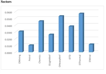
downwards accordingly in these sectors. Figure 2 displays the baseline 2025 shares of

electricity in total production cost for all sectors in which this share exceeds one percent.

Figure 2: Share of Electricity Cost in Total Baseline Production Cost 2025 – Selected Sectors

budget share parameters, as the assumed income elasticities of household demand for electricity for Kenya (see section 3 above) are well above unity across all household categories.

[image:28.595.69.440.353.612.2]

(29)

27

4.3. Lower Carbon Scenario

4.3.1. Scenario Specification

Considering alternative conceivable pathways towards a less carbon-intensive power mix, the

LCOE analysis for the GGDA project by Pueyo et al (2016) identifies geothermal electricity

generation as the most promising technology option for Kenya. This assessment is in line with

Kenyan government’s own assessment in the 10 Year Power Sector Expansion Plan:

“In Kenya, more than 14 high temperature potential sites occur along Rift Valley with an estimated potential of more than 10,000 MW. Other locations include Homa Hills in Nyanza, Mwananyamala at the Coast and Nyambene Ridges in Meru. The expansion to existing geothermal operations offers the least cost, environmentally clean source of energy (green) and highest potential to the country”. (Republic of Kenya, 2014:101).

The following simulation analysis contemplates a deliberately drastic scenario in which the

geothermal share in total domestic generation increases from 2018 onwards along a steep linear

schedule to reach 75 percent in 2025, so that the 2025 geothermal share is 23.6 percentage

points higher than in the baseline. The thermal share drops correspondingly from 35.2 percent

in the 2025 baseline to 11.6 percent (Table 6 and Figure 3a). The hydro and wind shares remain

unchanged. In absolute terms, this assumed expansion of geothermal electricity generation by

2025 is very close to the 10 Year Plan’s least-cost high growth scenario, in which geothermal

is projected to generate 26,000 GWh by 2024.

Table 6: Geothermal and Thermal Shares in Total Power Mix – Lower Carbon Scenario

(Percentage Shares)

Year Baseline Lower Carbon

Geothermal Thermal Geothermal Thermal

2015 50.0 17.5 50.0 17.5

2016 52.7 17.6 52.7 17.6

2017 53.9 18.9 53.9 18.9

2018 51.9 24.2 58.7 17.4

2019 50.7 27.6 62.4 15.9

2020 49.9 30.0 65.4 14.6

2021 50.8 30.8 68.7 12.9

2022 51.4 31.7 71.3 11.8

2023 51.7 32.6 73.2 11.2

2024 51.7 33.8 74.4 11.1

(30)

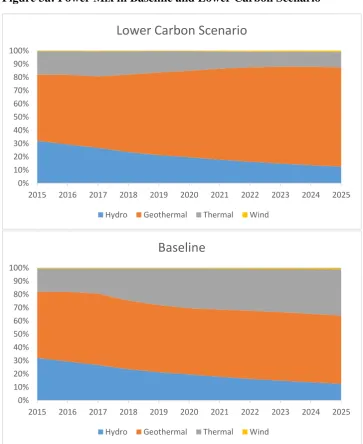
28 For a proper interpretation of this scenario it is important to emphasize that the falling share of

thermal does not imply an absolute contraction of thermal generation. Given the strong overall electricity demand growth, thermal generation still grows year on year, albeit at a lower rate

[image:30.595.70.434.218.663.2]

than in the baseline (Figure 3b).

Figure 3a: Power Mix in Baseline and Lower Carbon Scenario

0% 10% 20% 30% 40% 50% 60% 70% 80% 90% 100%

2015 2016 2017 2018 2019 2020 2021 2022 2023 2024 2025

Lower Carbon Scenario

Hydro Geothermal Thermal Wind

0% 10% 20% 30% 40% 50% 60% 70% 80% 90% 100%

2015 2016 2017 2018 2019 2020 2021 2022 2023 2024 2025

Baseline

(31)

[image:31.595.71.436.106.552.2]

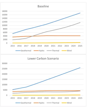
29 Figure 3b: Annual Electricity Generation in Baseline and Lower Carbon Scenario

(in GWh)

4.3.2. Results

The assumed gradual shift from high-cost thermal to lower-cost geothermal electricity

generation entails a notable drop in the effective average supply price relative to the baseline

scenario. As shown in Figure 4, in 2025 the domestic electricity price – here expressed relative

to the equilibrium wage of unskilled workers – is over 12 percent lower than in the baseline

scenario. The reduction in the cost of electricity affects the production costs and thus the supply

prices across all sectors and is more pronounced in sectors with a higher share of electricity in 0

2000 4000 6000 8000 10000 12000 14000 16000 18000

2015 2016 2017 2018 2019 2020 2021 2022 2023 2024 2025

Baseline

Geothermal Hydro Thermal Wind

0 5000 10000 15000 20000 25000 30000

2015 2016 2017 2018 2019 2020 2021 2022 2023 2024 2025

Lower Carbon Scenario

(32)

30 total cost (Figure 4) such as mining, the chemical industry and heavy manufacturing than in

[image:32.595.75.437.188.410.2]

sectors with a low power intensity.

Figure 4: Impact on Domestic Producer Prices – Lower Carbon Scenario 2025

(Percentage deviation of price relative to unskilled wage from 2025 baseline)

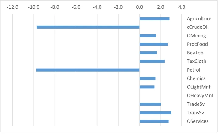
The assumed low carbon transition entails a strong reduction in fossil fuel imports. Both refined

petrol and crude oil imports drop by nearly ten percent in volume terms relative to the baseline

scenario towards 2025 (Figure 4). The indirect effect on crude oil imports arises due to the fact

that in the baseline scenario Kenya’s domestic petrol refining sector – which actually ceased

production in the second half of 2013 – is reactivated as envisaged in the 2015 National Energy

and Petroleum Policy Draft (Republic of Kenya, 2015) and as part of the aforementioned

LAPSSET flagship development. In the baseline projection this sector operates at a modest

scale using imported crude oil, with a negligible 2025 baseline contribution to GDP and total

employment.

As Kenya remains a net importer of fossil fuels in the baseline scenario, the drop in the fossil

fuel import bill is associated with a real exchange rate appreciation on the order of 0.7 percent.

The real appreciation lowers in tendency the prices of imports relative to domestically produced

goods from the perspective of domestic residents. This induces a substitution effect towards

imports for commodities in cases where the exchange rate effect dominates the simultaneous

drop in the prices of domestic output due to the electricity cost reduction in the new

equilibrium. This substitution effect affects both imports of final goods and intermediate inputs.

-14.0 -12.0 -10.0 -8.0 -6.0 -4.0 -2.0 0.0

(33)

31 A further positive effect on imports across all final goods arises due the positive aggregate real

income effects associated with the shift towards lower-cost electricity generation shown below.

Thus, Figure 5 shows moderate welfare-raising increases in the import quantities relative to

baseline levels for most traded non-fuel goods and services and these are generally more

pronounced for the commodity groups with smaller domestic supply price reductions according

[image:33.595.72.435.291.513.2]

to Figure 4.

Figure 5: Impact on Real Import Volumes by Commodity Group – Lower Carbon Scenario 2025

(Percentage deviation from 2025 baseline)

Note: This figure excludes commodity groups with negligible shares in Kenya’s total imports.

On the export side, the real exchange rate appreciation effect per se reduces in tendency the

price of exports relative to the price obtained in the domestic market from the viewpoint of

domestic producers, and thus shifts the optimal profit-maximizing output mix between export

and home market production in favour of the latter. Correspondingly, Figure 6 reports moderate

drops in export quantities for most sectors. An exception is heavy manufacturing, which is the

sector with the highest electricity cost share. In this case, the cost reduction effect dominates

the exchange rate effect, so that exports expand.

The trade effects shown in Figure 5 and 6 can also be explained from a balance-of-payments

perspective: The reduction in the fossil fuel import bill relaxes the balance-of-payments

-12.0 -10.0 -8.0 -6.0 -4.0 -2.0 0.0 2.0 4.0

Agriculture

cCrudeOil

OMining

ProcFood

BevTob

TexCloth

Petrol

Chemics

OLightMnf

OHeavyMnf

TradeSv

TransSv

(34)

32 constraint as it allows domestic residents to enjoy simultaneously an increase in real imports

and a higher share in domestically produced output, as less of that output needs to be shipped

abroad to pay the import bill.

Figure 6: Impact on Real Export Volumes by Commodity Group – Lower Carbon Scenario 2025

Note: The figure excludes commodity groups for which both the baseline share in total export revenue is small (<2.5 percent) and the export/output share is small (<10 percent).

The equilibrium impact on real gross output by production sector for 2025 compared to the

baseline scenario is shown in Figure 7. The sectoral employment effects have the same

direction and broadly the same orders of magnitude, and are therefore not separately plotted.

Not surprisingly, in percentage terms the effect on the size of the small domestic oil refinery

sector in relation to the baseline is most pronounced as the demand growth for fuel by thermal

power plants slows down. However in relation to total employment the associated employment

reallocation effects are tiny. The domestic power sector expands as the drop in electricity prices

induces additional demand.

It is worth emphasizing that no sector contracts in absolute terms and thus no sector sheds

existing workers along the dynamic scenario time path. A negative-signed output effect in

Figure 7 merely indicates that the sector grows at a lower rate and that new workers are hired

a slower pace than in the baseline scenario. E.g., while the domestic refining sector at the 2025

-3.0 -2.5 -2.0 -1.5 -1.0 -0.5 0.0 0.5 1.0 1.5

Agriculture

Forestry

OMining

ProcFood

BevTob

TexCloth

Chemics

OLightMnf

OHeavyMnf

TransSv

(35)

33 endpoint of the simulation horizon is projected to be nearly 10 percent smaller than in the

baseline scenario for the same year, the sector is still 127 percent larger in 2025 than in 2027.

In line with economic theory, the real exchange appreciation shifts in tendency productive

resources from traded to non-traded activities. Among the non-power sectors that expand

relative to baseline are all sectors that have simultaneously negligible or small export / output

shares and negligible or little competition from imports in their domestic market, such as

construction services the fishery sector, and trade services. In contrast, the small domestic

mining sector with its baseline export-output ratio of over 75 percent and an import share of over 50 percent in Kenya’s domestic demand for mining products is squeezed noticeably as mining exports drop and mining imports rise. The sectors that expand despite relatively high

trade shares are heavy manufacturing are heavy manufacturing, which – as noted earlier – are

among the most electricity-intensive sectors and thus benefit disproportionally from the

reduction in energy input costs. However, the main message from Figure 7 is that the effects

of the assumed low carbon transition on the sectoral composition of output and employment

are very moderate.

Figure 7: Impact on Real Output by Sector – Lower Carbon Scenario 2025

-10.0 -8.0 -6.0 -4.0 -2.0 0.0 2.0 4.0

Agriculture

Forestry

Fishing

Mining

ProcFood

BevTob

TexCloth

Petrol

Chemics

OLightMnf

OHeavyMnf

Electricity

Construction

TradeSv

TransSv

(36)

34 The real resource savings associated with the switch to a lower-cost mode of electricity

generation is reflected in a moderately positive transitory effect on GDP growth as shown in

Figure 8. Like in a standard Solow growth model, the long-run growth rate in this multi-sectoral

dynamic CGE model is exogenously determined by the sum of the aggregate growth rate of

technical progress and the labour force growth rate. As these rates remain the same as in the

baseline, the annual GDP growth rate in a hypothetical dynamic long-run equilibrium without

further changes in exogenous parameter would eventually converge back to the baseline growth

rates, yet the positive effect on the level of GDP is of course permanent along such a steady

state path. The cumulative effect of the small annual growth rate increments reported in Figure

8 over the period 2018 to 2025 entails that the level of real GDP by 2025 is 1.1 percent higher

than in the baseline scenario.

Figure 8: Annual Growth Rate of Real GDP – Baseline and Low Carbon Scenario

(in Percent)

Turning to the effects on the functional income distribution – that is the distribution of primary

income by type of factor – Figure 9 displays the impacts on real factor prices (i.e. nominal

factor prices deflated by the consumer price index) in 2020 and 2025 relative to the baseline

level in the corresponding year. By 2025 the real returns to all factors except mineral resources

are slightly higher than in the baseline. Capital returns rise relative to labour wages and the

wage gap between skilled and unskilled increases marginally. 0.00

1.00 2.00 3.00 4.00 5.00 6.00 7.00 8.00

2018 2019 2020 2021 2022 2023 2024 2025

6.10

7.50 7.50 7.50 7.50 7.50 7.50 7.50

6.47

7.82 7.78 7.69 7.66 7.63 7.61 7.59

(37)

35 The differential factor price effect arise from factor intensity differentials between sectors that

grow quicker and sectors that grow slower than in the baseline (recall Figure 7): On balance,

the higher-growing sectors as a group are relatively skill- and capital-intensive and thus their

additional factor input demand drives up capital returns and skilled wages more than unskilled

wages.

The natural resource rent drop is due to the growth slow-down of the domestic mining sector

which is the sole user of the mineral endowment factor in the model. The reason for the reversal

of the effect on agricultural land rents is related to the fact that electricity use in agriculture is

initially very low but grows over time with technical progress and the rise in rural access rates.

Thus, agriculture initially benefits very little from the drop in electricity prices while being hit

by the exchange rate appreciation effect on agricultural exports and imports (Figure 5 and 6).

As a result, agricultural output drops marginally (by 0.1 percent) below baseline levels over

the initial period up to 2020 but then recovers subsequently (and ends up 0.1 percent above

base level by 2025) as the direct and indirect23 input cost reduction effects become more

pronounced over time.

For households with a single source of factor income, Figure 9 directly indicates the direction

of the effects on total factor income. Figure 10 shows the implications for mixed-income

households with factor income mixes equal to the income compositions of the four household

categories the benchmark SAM. Both lower and higher income households gain. However,

since the urban and rural high-income groups have higher shares of capital and skilled labour

in their total income mix than the low-income groups, the former groups gain disproportionally.

In other words, as far as this rather coarse-grained distributional analysis based on outdated

underlying raw data goes, the low-carbon transition has a pro-poor effect in an absolute or “weak” sense (namely that the poorer households are better off than in the baseline), but is not pro-poor in a relative or “strong” sense (i.e. the poorer households do not gain

disproportionally).24

23_{E.g. the drop in chemical fertilizer prices.}

(38)

36 Figure 9: Impact on Factor Returns – Low Carbon Scenario

(Percentage deviation of factor prices relative to CPI baseline level 2020 and 2025)

Figure 10: Impact on Real Household Income – Low Carbon Scenario

(Percentage deviation from Baseline level 2020 and 2025)

-1.5 -1.0 -0.5 0.0 0.5 1.0 1.5 2.0

Unskilled Labour

Skilled Labour

Land

Capital