Manipulating a stated choice experiment

Munich Personal RePEc Archive

Manipulating a stated choice experiment

Fosgerau, Mogens and Börjesson, Maria

Technical University of Denmark, Denmark, Royal Institute of

Technology, Sweden

2015

Online at

https://mpra.ub.uni-muenchen.de/67053/

Manipulating a stated choice experiment

Mogens Fosgerau

Technical University of Denmark, Denmark

Royal Institute of Technology, Sweden

[email protected]

Maria Börjesson

Royal Institute of Technology, Sweden

[email protected]

September 24, 2015

Abstract

This paper considers the design of a stated choice experiment intended to measure the marginal rate of substitution (MRS) between cost and an attribute such as time using a conventional logit model. Focusing the exper-imental design on some target MRS will bias estimates towards that value. The paper shows why this happens. The resulting estimated MRS can then be manipulated by adapting the target MRS in the experimental design.

JEL: C8, C9, C25

1

Introduction

This paper considers a stated choice experiment designed to measure the marginal rate of substitution (MRS) between cost and another attribute of the choice alter-natives. We present a case where the design is centered on some target MRS and where the MRS is estimated by applying a conventional logit model. We demon-strate that if the random individual response heterogeneity is mainly driven by heterogeneity of the MRS rather than by response errors, then the estimated MRS will tend to be biased towards the target. This bias hinges on misspecification of the logit model, which has constant marginal utilities and additive random resid-uals. Thus, this bias will tend to confirm the target MRS and may thus not be informative about consumer preferences.

Seasoned choice experiment designers probably know this already. The ob-jective of this paper is to make clear how the mechanism works and to make this insight more widely accessible.

Stated choice experiments are used within a range of applied fields of eco-nomics, including energy, transportation, health, tourism, agricultural and envi-ronmental economics. They are also used by consultants in a variety of contexts and in marketing. The mechanism explored in this paper may not only be present in stated choice data, but also when the MRS is estimated on revealed preference data.

The mechanism described in the present paper should not be confused with other sources of bias on the MRS inferred from stated choice data. The choice experiment can influence the output for a number of reasons. Many cognitive processes are at play when people make decisions, typically simplified by various decision rules, heuristics, implying that the experimental design can influence the result (Hensher, 2014;Leong and Hensher,2012). There are empirical (Bliemer and Rose, 2011) and theoretical indications (Burgess and Street, 2005; Sandor

and Wedel, 2005) that attribute levels and the order of them within the

experi-ment influence output (seeRose and Bliemer,2014, for a review). De Borger and Fosgerau(2008) andHess et al.(2008) show that preference asymmetries such as different valuation of gains or losses, and reference effects influence respondent’s stated choices, with De Borger and Fosgerau(2008) linking these phenomena to prospect theory (Tversky and Kahneman, 1991). In particular, the value of time from stated choice experiments has been found to depend on the size and sign of the attribute differences between the alternatives. A commonly found sign effect is that gains are valued less than losses; this is called loss aversion. Size effects refer to cases where the estimated MRS is found to depend on the size of the at-tribute difference between alternatives (e.g., Mackie et al.,2001;Hultkrantz and

savings.

Adaptive design techniques can introduce bias in the estimated MRS through yet another mechanism, namely that attribute levels and unobserved heterogene-ity in the respondents preferences become correlated (Bradley and Daly, 1993). Adaptive designs then lead to a self-imposed endogeneity problem, violating the statistical assumptions underlying standard models, and making subsequent sta-tistical inference invalid.

There is evidence that stated choices are sometimes subject to hypothetical bias (Harrison, 2014). In the context of risky choices, nonlinearities regard-ing attitudes and perceptions of risks imply that the design of the experiment in terms of risk levels and presentation of those influence the choices (Bates et al.,

2001;Liu and Polak,2007;Borjesson and Eliasson,2011;Loomes and Blackburn,

2014).These other potential sources of bias are not in focus in this paper.

The mechanism we discuss in the present paper relates to the boundary value design approach (Fowkes and Wardman, 1988). The idea of this design approach is to choose boundary or trade-off values within a range where the analyst think the MRS distrubution is located. Fowkes and Wardman point out that the boundary values should cover a reasonable range of potential variation in taste and uncer-tainty, but that it is often desirable to have them closer together in the range where the actual values are expected to be located. An implication of our results is that the boundary value approach should be avoided, since it runs the risk of biasing the estimated MRS toward the chosen boundary values. Moreover, it is not suited to models that account for preference heterogeneity.

A remedy to avoid the bias arising from the misspecification of the logit model is to explore the error structure of the data, using non-parametric techniques, before defining a parametric model. If such analysis indicates heterogeneity in the MRS, the parametric model should allow for heterogeneity in the MRS. The choice of parametric distribution for the MRS is crucial and should be tested ( Fos-gerau and Bierlaire,2007;Fosgerau and Mabit,2013).

To estimate the distribution of the MRS, a key condition is that the full dis-tribution of the MRS is uncovered by the data. If this condition is not met, then the estimates of the mean and other moments of the MRS distribution have to rely on assumptions about the shape of the distribution in the range where it cannot be identified by the data. Such assumptions are hard to verify. Fosgerau (2006) shows that when the tail of the MRS distribution is not revealed, then sthe choice of parametric distributions can result in arbitrarily high estimates of the mean MRS. The resulting estimated of the mean MRS will depend on the parts of the distribution that are extrapolated outside the range of data.

the random MRS model, and describes the mechanism that tends to bias the esti-mated MRS. Section 4describes the experimental design used in the simulation exercise in section 5. Section 6 uses part of the Danish value of time data to empirically validate the theoretical predictions of section3. Section7concludes.

2

Choice setup and the model to estimate

The context of a trip is used for concreteness. The alternatives can be different routes by some mode of transportation, for example; section6uses data concern-ing rail trips. Each subject is asked to choose between two alternatives for a trip and each route is characterized by an associated monetary cost and a travel time.

This setting can be used to reveal the subjects’ rate of substitution between travel time and cost. By design, one route will be faster but also more expensive than the other. With everything else being equal, subjects reveal through their choices whether their willingness to pay for the time saving associated with the faster route is greater or smaller than the cost difference between the two routes.

The canonical model for this situation is the logit model with the founda-tion in the theory of consumer demand developed by McFadden (1974). The conventional and widely used specification of the binary logit model in this set-ting uses indirect utilities for the two alternatives that are linear indices vij =

cij+ tij+ 1fj=2g+"ij, where subscriptiindexes individuals,j = 1;2indexes

choice alternatives, cij is the travel cost for individualiin alternativej with

cor-responding marginal utility , tij is the travel time with corresponding marginal

utility , is a constant specific to alternative2 and"ij are i.i.d. extreme value

type 1 random residuals. The marginal utilities ; are expected to be negative. Each individual chooses the alternative yielding the highest indirect utility. Then the probability that alternative1is chosen is

pi1 =

e ci₁+ ti₁ e ci₁+ ti₁ +e ci₂+ ti₂+

= 1

1 +e ci+ ti+ ; (1)

where ci = ci2 ci1 and ti = ti2 ti1. The marginal rate of substitution

between time and cost in this model is = .

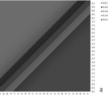
Figure1shows the shape of the logit probabilityp1 as a function of( c; t).

In the quadrant shown, alternative 1 has a lower travel cost but a longer travel time than alternative 2 ( ci is positive and ti is negative). In the light gray

area in the upper left corner the probability of choosing the cheaper alternative 1 is high (ranging from 0:8 to 1). In the darker area in lower right corner the probability is low (ranging from 0to0:2). The point of the figure is to show that the probability is constant on parallel straight lines in the ( c; t)-plane. From the logit probability (1) we see that constantp1implies that c+ t+ =C,

whereCis a constant given by probabilityp1. This implies c=C t,

which shows that the equiprobability lines have the constant slope = .

Keeping the ratio = fixed, the distance between equiprobability lines de-creases as and increase in absolute value. This is easily seen on the vertical

c-axis in the figure, along which t = 0. The distance between the equiproba-bility lines equals C, where C is a function of the difference in probability be-tween the lines ( p1) which is 0.2 in the figure. Hence, a larger , implies a larger

distance between the lines. On the t-axis the distance between the equiproba-bility lines equals C.

The equiprobability lines can be shifted perpendicularly by changing . The probability traces out a logistic distribution in the direction perpendicular to the equiprobability lines.

Fitting the logit model to responses to( c; t)by estimating( ; ; )amounts to determining the best slope = of equiprobability lines, determining the scale of ( ; )to match the distance between equiprobability lines and determining to match the location of the equiprobability lines.

3

A more realistic data generating process

When fitting the standard logit model described in the previous section to data, the modeler makes the assumption that all the response heterogeneity in the data arises from response error and none from variation in the MRS. To illustrate how the logit model may bias the result if this assumption does not hold, we continue by making the assumption in the other extreme: that all the response heterogeneity in the data arises from variation in MRS and none of it arises from response error. We assume that this data is the result of the choice generation process ruled by the random MRS model proposed byCameron and James(1987).

In the random MRS model, individuals each have a MRSwi, which has some

absolutely continuous population distribution . Individual i evaluates alterna-tives with the generalized cost cij +witij and chooses the alternative with the

0.1 0.5 0.9 1.3 1.7 2.1 2.5 2.9 3.3 3.7 4.1 4.5 4.9 5.3 5.7 6.1 6.5 6.9 7.3 7.7 8.1 8.5 8.9 9.3 9.7

‐

0.1 _‐0.5 _‐0.9 _‐1.3 _‐1.7 _‐2.1 _‐2.5 _‐2.9 _‐3.3 _‐3.7 _‐4.1 _‐4.5 4.9_{‐ ‐}5.3 _‐5.7 _‐6.1 _‐6.5 _‐6.9 7.3_{‐ ‐}7.7 _‐8.1 _‐8.5 _‐8.9 _‐9.3 _‐9.7



c



t

0.8‐1

0.6‐0.8

0.4‐0.6

0.2‐0.4

0‐0.2

chosen by individualiis ^

pi1 = P(ci1+witi1 < ci2+witi2)

= P( wi ti < ci)

= 8 <

:

ci

ti ti <0

1 ci

ti ti >0

(2)

The difference between this model and (1) is that all response heterogeneity here is captured bywi, while there is no"added to capture random error.

This model is similar to the transfer price model of HensherHensher(1976) , which assumes that cu +T P ca = a0 +a1(tu ta), where c is travel, t

is travel time, uindicates the usual mode, a indicates alternative mode, and the transfer price T P is defined as ’the amount of cost change that would have to occur in the usual mode journey for the individual to consider an alternative mode of transport’.

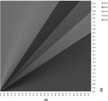
Figure2 shows the probability that alternative 1is chosen against ( c; t), using as example a lognormal distribution for . From (2), we have that ci =

C ti, where C is constant for a given probability. Hence, the probability is

constant on rays from the origin in ( c; t)-space as illustrated in the figure. From (2) we also see that the slope of the equiprobability lines increases in p1

in the quadrant shown in the figure (where ti < 0). The equiprobability lines

have a large slope in the light area in the upper left corner where the probability of choosing the alternative1is high (ranging from 0.8 to 1). In the dark gray area in the lower right corner, where the probability is low (ranging from 0 to 0.2), the equiprobability lines have smaller slope.

Previous studies suggest that the random MRS model is a better description of the true data generating process than the logit model (1): Fosgerau(2007) and

Borjesson et al. (2012) use nonparametric techniques to distinguish between the

logit and the random MRS choice generating processes, with data from the Danish and the Swedish national value of time studies, respectively. Both studies find clear evidence in favor of the random MRS model. A part of the Danish dataset is used in section 6.

4

A bad experimental design

0.1 0.5 0.9 1.3 1.7 2.1 2.5 2.9 3.3 3.7 4.1 4.5 4.9 5.3 5.7 6.1 6.5 6.9 7.3 7.7 8.1 8.5 8.9 9.3 9.7

‐

0.1 _‐0.5 _‐0.9 _‐1.3 _‐1.7 _‐2.1 _‐2.5 _‐2.9 _‐3.3 _‐3.7 _‐4.1 _‐4.5 4.9_{‐ ‐}5.3 _‐5.7 _‐6.1 _‐6.5 _‐6.9 7.3_{‐ ‐}7.7 _‐8.1 _‐8.5 _‐8.9 _‐9.3 _‐9.7



c



t

0.8‐1

0.6‐0.8

0.4‐0.6

0.2‐0.4

0‐0.2

shall see what happens when a data generating process that really is the random MRS model of Section3meets a modeler who has the logit model of Section2in mind. This is the core insight of this paper.

Say that the experimental designer assumes a constant MRS across the popu-lation and has a target MRS in mind, denotedw^. He1 _{may first select time}

differ-ences tifrom some range. The range would be chosen to yield time differences

that are noticeable and that subjects can accept as being realistic. Next, he may select corresponding values of cost differences ci that are near w t^ i, but with

an equal mix of values that are larger and smaller such that the design has points ( ci; ti) that are centered on the ray with slope w^. A common rationale for

such a design strategy is that it should ensure that the MRS = (assumed con-stant by the designer) is estimated with high precision provided it is close to w^. Having collected responses to this design, the final point in this methodology is to fit a logit model as in (1) to these data.

Under the maintained and plausible assumption that the main source of het-erogeneity is actually random MRS with some distribution, the expected response will be similar to Figure2. By design, there will be only data near the target ray and the expected response will be roughly constant.

If the sample is sufficiently large, then the estimated logit model (or a similar model) will approximate this shape. Therefore the estimated logit model will have constant probability on lines that have slope close to the target MRS and thus the estimated MRS will be close to the target. This is, of course, extremely prob-lematic, since the point of the exercise is to estimate the MRS of experimental subjects and not the target MRS of the experimental designer. The scale of the coefficients ; is determined by the slope of the response surface in the perpen-dicular direction while the constant adjusts to match the estimated probability to the observed.

5

Simulation exercise

The theoretical predictions made in section 2 and section 3 are now validated in a small simulation exercise. In the simulation exercise we adopt the choice generation process described in section 3, the random MRS model. We generate five datasets by applying an experimental design as discussed in section4. In the simulation of each of the five data sets we assume a different target MRSw^when generating the experimental design. The standard logit model (1) is then estimated on the five simulated datasets, such that one MRS estimate is achieved for each dataset and target MRS.

1

Table 1: Estimation results, simulation data, standard errors in parentheses

Target MRS Estimated MRS

0.5 -0.246 (0.062) -0.162 (0.037) -0.613 (0.28) 0.662 1 -0.149 (0.026) -0.159 (0.030) 0.174 (0.24) 1.064 2 -0.080 (0.015) -0.175 (0.035) 1.426 (0.28) 2.205 3 -0.068 (0.013) -0.224 (0.043) 2.248 (0.36) 3.292 4 -0.056 (0.012) -0.259 (0.054) 3.022 (0.45) 4.598

More specifically, a choice experiment was designed by first fixing a target MRS. Time differences tiwere sampled from a uniform distribution on[10;20]

and the cost differences were set to a the target MRS times a random noise term sampled from a uniform distribution on[0:8;1:2].

A dataset was then generated where 2000 individuals make one choice each with an MRS drawn from a standard lognormal distribution. Applying the binary logit model (1) the MRS is then estimated from the generated dataset. The whole procedure is then repeated four times assuming different target MRS in the design of the choice experiment.

Table1reports the logit estimation results, including the estimated MRS =

corresponding to each of the five target MRS. Evidently, it is possible to generate estimated MRS that are quite close to the target over a wide range. The parameters of interest and are estimated with good precision, which would not lead one to suspect problems. This happens even though the model, by construction, is misspecified.

6

Empirical test

The empirical test uses data from a Danish value of time study (Fosgerau et al.,

2007). The dataset concerns binary choices between train trips differentiated by travel time and cost. The design was created pivoting around the travel time and cost of actual train trips undertaken by subjects. Eight choice situations were gen-erated for each subject by first drawing two absolute travel time differences from a set. Second, eight MRS were drawn from the interval [3:200] Danish Kroner (DKK) per hour2_{, using stratification to ensure that all subjects were presented}

with both low and high values. The absolute cost difference was then found for

2

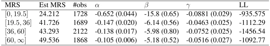
Table 2: Estimation results, rail data, standard errors in parentheses

MRS Est MRS #obs LL

[0;19:5] 24.212 1728 -0.652 (0.044) -15.8 (0.65) -0.0881 (0.029) -935.575 [19:5;36] 41.726 1689 -0.147 (0.020) -6.14 (0.56) -0.0463 (0.025) -1112.29 [36;60] 43.293 2122 -0.138 (0.017) -5.98 (0.80) -0.0752 (0.025) -1456.54 [60;1] 49.536 1868 -0.105 (0.006) -5.18 (0.52) -0.0516 (0.027) -1092.77

each choice situation by multiplying the absolute time difference by the MRS. Third, the sign of the cost and time differences relative to the reference were de-termined such that they were opposite and such that each of the four possible permutations was used twice. The differences were added to the reference to get the numbers that were presented to subjects on screen. The sequence of choice situations was randomly scrambled. Travel costs were rounded to the nearest 0.5 DKK. The data have been trimmed prior to analysis by removing the 5% of ob-servations having the largest journey times and time and cost differences.3

The choice situations in these data have a wide range of implicit MRS. They can therefore be used to simulate the effect of using a narrower range of MRS centered on different target MRS. The data are thus split according to quartiles of the MRS implicit in choice situations and a model is estimated for each quartile. This simulates designs that are based on different intervals of MRS. The following table shows the results of estimating binary logit models on these data. The data in each split are pooled and standard errors are not corrected for repeated obser-vations. Our interest is just to see how the estimated MRS can be manipulated.

The results in Table2show that the estimated MRS does change in the appro-priate direction as the MRS design interval is changed and that there is a factor two difference between the highest and the lowest estimated MRS. This shows that the approach outlined above leads to estimation results that are strongly in-fluenced by the target MRS. As in the simulation exercise, the precision of the estimates is good, which does not reveal that the model is misspecified.

The relationship between estimated and target MRS is not as tight as in the simulation. This is unsurprising since the simulation model was created to pre-cisely deliver the desired effect.The simulation model, however, is not a perfect representation of the choice behavior of real subjects, and we do expect that some response heterogeneity arises from other sources than variation in MRS in real data.

7

Concluding remarks

There is empirical evidence indicating that a substantial part of the response het-erogeneity in stated choice experiments arises from variation of the MRS in the population. That, in combination with an SP design based on a target MRS and in combination with a misspecified model, will lead to bias. This can be a severe problem.

We have illustrated the problem in a very simple setting with just two alter-natives and two attributes and a naive SP design. While this is very simple, it is close to what is sometimes done, in research and in consultancy projects. Of course current state-of-the-art design techniques are much more sophisticated, see

Rose and Bliemer(2009) for an overview. We do, however, hope that the intuition one may gain from the examples we have presented in this paper will be useful when working with more advanced design methods. It seems to be an open ques-tion to which extent various types of designs and consequent model estimaques-tion are robust against misspecification.

Extrapolating from our results, it is possible to offer some guidance. One gen-eral point is that it is a very good idea to perform specification testing of estimated models. We have seen that it is not sufficient to examine the precision of parame-ter estimates. It is possible to have quite precise estimates from a model that is completely misspecified.

In order to be able to do specification testing, it is important that there is suffi-cient variation in the data that allows potential misspecification to detected. This provides an argument for SP designs with wide attribute ranges. Wide attribute ranges are also useful for identification of parameter distributions, where the tribution of willingness-to-pay parameters is of particular interest. Where the dis-tribution of a random MRS is of interest, then experimental design should allow nonparametric identification of that distribution. Our results illustrate the impor-tance of using SP designs that are robust in the sense that they will allow the identification of a range of models.

Analysis of SP data often uses the plain logit model similar to (1) as a start-ing point and elaborates from that. In principle, this model can be generalised into any other model, for example adding (many) random parameters (McFadden and Train, 2000). In practice, however, this is never possible since datasets are always finite and mostly not that large. It is then a better idea to begin from a parsimonious model that describes the main features of the data. Depending on the circumstances, this could be a model where the basic source of randomness is random MRS rather than random noise. Non-parametric tools exist that can assist in choosing a base model.

structure of the data that matters, not how they were generated. We note also that it is not essential that the sign of the random MRS is known, the results in section

3can be extended to cases where the sign of the random MRS is negative or where it may attain both positive and negative values.

We hope that these results will inspire further research on SP design and analy-sis.

8

Acknowledgements

We thank Glenn Harrison and Stefan Mabit for comments. Mogens Fosgerau has received financial support from the Danish Strategic Research Council.

References

Bates, J., Polak, J., Jones, P. and Cook, A. (2001) The valuation of reliability for personal travelTransportation Research Part E37(2-3), 191–229.

Bates, J. and Whelan, G. (2001) Size and sign of Time SavingsITS Working Paper

(561).

Bliemer, M. C. J. and Rose, J. M. (2011) Experimental design influences on stated choice outputs: An empirical study in air travel choiceTransportation Research Part A: Policy and Practice45(1), 63–79.

Borjesson, M. and Eliasson, J. (2011) On the use of â ˘AIJaverage delayâ ˘A˙I as a measure of train reliabilityTransportation Research Part A: Policy and Practice

45(3), 171–184.

Borjesson, M., Fosgerau, M. and Algers, S. (2012) Catching the tail: Empirical identification of the distribution of the value of travel timeTransportation Re-search Part A: Policy and Practice46(2), 378–391.

Bradley, M. and Daly, A. (1993) New issues in stated preferences research Tech-nical report21st PTRC Summer Annual Meeting Manchester, U.K.

Burgess, L. and Street, D. J. (2005) Optimal designs for choice experiments with asymmetric attributes Journal of Statistical Planning and Inference

134(1), 288–301.

De Borger, B. and Fosgerau, M. (2008) The trade-off between money and time: a test of the theory of reference-dependent preferencesJournal of Urban Eco-nomics64(1), 101–115.

Fosgerau, M. (2006) Investigating the distribution of the value of travel time sav-ingsTransportation Research Part B: Methodological40(8), 688–707.

Fosgerau, M. (2007) Using nonparametrics to specify a model to measure the value of travel time Transportation Research Part A: Policy and Practice

41(9), 842–856.

Fosgerau, M. and Bierlaire, M. (2007) A practical test for the choice of mixing distribution in discrete choice modelsTransportation Research Part B: Method-ological41(7), 784–794.

Fosgerau, M., Hjorth, K. and Vincent Lyk-Jensen, S. (2007) The Danish Value of Time Study - Final ReportTechnical reportwww.dtf.dk.

Fosgerau, M. and Mabit, S. L. (2013) Easy and flexible mixture distributions Eco-nomics Letters120(2), 206–210.

Fowkes, T. and Wardman, M. (1988) The Design of Stated Preference Travel Choice Experiments: With Special Reference to Interpersonal Taste Variations

Journal of Transport Economics and Policy22(1), 27–44.

Harrison, G. W. (2014) Real choices and hypothetical choices Handbook of Choice ModellingEdward Elgar Publishing pp. 236–254.

Hensher, D. (2014) Attribute processing as a behavioural strategy in choice mak-ing Edward Elgar pp. 268–289.

Hensher, D. A. (1976) The Value of Commuter Travel Time Savings: Empirical Estimation Using an Alternative Valuation Model Journal of Transport Eco-nomics and Policy10(2), 167–176.

Hess, S., Rose, J. M. and Hensher, D. A. (2008) Asymmetric preference forma-tion in willingness to pay estimates in discrete choice models Transportation Research Part E: Logistics and Transportation Review44(5), 847–863.

Hultkrantz, L. and Mortazavi, R. (2001) Anomalies in the Value of Travel-Time ChangesJournal of Transport Economics and Policy35(2), 285–300.

Liu, X. and Polak, J. (2007) Nonlinearity and Specification of Attitudes Toward Risk in Discrete Choice Models Transportation Research Record: Journal of the Transportation Research Board2014, 27–31.

Loomes, G. and Blackburn, S. (2014) Towards a more complex model of risky choice Edward Elgar pp. 73–98.

Mackie, P., Jara-Diaz, S. and Fowkes, A. (2001) The value of travel time savings in evaluationTransportation Research Part E: Logistics and Transportation Re-view37(2-3), 91–106.

McFadden, D. (1974) Conditional Logit Analysis of Qualitative Choice Behaviour

Frontiers in EconometricsAcademic Press New York pp. 105–142.

McFadden, D. and Train, K. (2000) Mixed MNL Models for discrete response

Journal of Applied Econometrics15, 447–470.

Rose, J. and Bliemer, M. (2014) Stated choice experimental design theory: the who, the what and the why Edward Elgar pp. 152–177.

Rose, J. M. and Bliemer, M. C. J. (2009) Constructing Efficient Stated Choice Experimental DesignsTransport Reviews29(5), 587–617.

Sandor, Z. and Wedel, M. (2005) Heterogeneous Conjoint Choice DesignsJournal of Marketing Research42(2), 210–218.

Tversky, A. and Kahneman, D. (1991) Loss Aversion in Riskless Choice: A Reference-Dependent Model The Quarterly Journal of Economics