Munich Personal RePEc Archive
Qml inference for volatility models with
covariates
Francq, Christian and Thieu, Le Quyen
Crest and Universté de Lille, Université Pierre et Marie Curie
March 2015
Online at
https://mpra.ub.uni-muenchen.de/63198/
Qml inference for volatility models with covariates
Christian Francq
Le Quyen Thieu
∗CREST and Université de Lille, Université Pierre et Marie Curie.
Abstract
The asymptotic distribution of the Gaussian quasi-maximum likelihood esti-mator (QMLE) is obtained for a wide class of asymmetric GARCH models with exogenous covariates. The true value of the parameter is not restricted to belong to the interior of the parameter space, which allows us to derive tests for the signifi-cance of the parameters. In particular, the relevance of the exogenous variables can be assessed. The results are obtained without assuming that the innovations are independent, which allows conditioning on different information sets. Monte Carlo experiments and applications to financial series illustrate the asymptotic results. In particular, an empirical study demonstrates that the realized volatility is an helpful covariate for predicting squared returns, but does not constitute an ideal proxy of the volatility.
Keywords: APARCH model augmented with explanatory variables, Boundary of the
param-eter space, Consistency and asymptotic distribution of the Gaussian quasi-maximum likelihood estimator, GARCH-X models, Power-transformed and Threshold GARCH with exogenous co-variates.
1
Introduction
The GARCH-type models are of the form
εt=σtηt, (1)
∗Corresponding author: Le Quyen Thieu, Université Pierre et Marie Curie, France. Telephone:
where the squared volatility σ2
t is the best predictor ofε2t given a certain information set
Ft−1 available at time t. More precisely, it is assumed that E(εt2 | Ft−1) = σt2 > 0, or
equivalently that σt>0, σt∈ Ft−1 andE(ηt2 | Ft−1) = 1. For the usual GARCH models,
Ft−1 is simply the sigma-field generated by the past returns{εu, u < t}, and the volatility
has a parametric formσt=σ(εu, u < t;θ0), whereθ0 is a vector of parameters. It is how-ever often the case that some extra information is available, under the form of a vector
xt−1 of exogenous covariates, such as the daily volume of transactions, or high frequency
intraday data, or even series of other returns. It is natural to try to take advantage of
the extra information, in order to improve the prediction of the squares. To incorporate
the information conveyed by {xu, u < t}into Ft−1, researchers have considered GARCH
models augmented with additional explanatory variables, the so-called GARCH-X
mod-els, which are of the form σt = σ(εu,xu, u < t;ϑ0), where ϑ0 is a vector of parameters including a parameter θ0 specific to the past returns and a parameter π0 related to the
exogenous covariates (see e.g. Engle and Patton (2001) and the references therein).
In practice, the difficulties are the choice of the parametric form (as illustrated by
Bollerslev (2008), there exists a plethora of GARCH formulations) and the estimation
of the parameter ϑ0. The two problems are closely related. For GARCH, as well as
for GARCH-X models, the coefficients are generally positively constrained, and tests of
nullity of some components of ϑ0 help to find a parsimonious GARCH-X formulation.
The usual estimator of the GARCH models is the quasi-maximum likelihood estimator
(QMLE), which does not require to specify a particular distribution for the error termηt.
The consistency of the QMLE does even not require that(ηt)be iid, which is particularly
relevant for GARCH-X models (see Remarks 3 and 4below). The asymptotic normality
however requires that the true value of the parameter belongs to the interior of the
parameter space, which is generally not the case when components of ϑ0 are equal to
zero.
Questions that seem particularly relevant in the GARCH-X framework are: is it really
useful to introduce covariates in the volatility? which covariates should we add to Ft−1?
how many lagged values should we consider in the GARCH formulation? Some researchers
and practitioners even reject any GARCH model, and consider that the realized volatility
the following question: is it necessary to include the past returns {εu, u < t} in the
volatility when the sequence (xt) of the realized volatilities is available?
Each of these questions can be discussed by testing the nullity of certain components
of ϑ0. It is thus of interest to study the behaviour of the estimator ϑbn of ϑ0 when this parameter may stand at the boundary of the parameter space. To our knowledge, this
problem has not yet been explicitly considered for GARCH-X models. This will be the
focus of this paper. We now present the class of GARCH-X that we will consider, and
then we detail the main objectives of the paper.
1.1
The model
Letx+ = max(x,0)and x−
= max(−x,0). We consider the model defined by
εt=h1t/δηt
ht=ω0+Pqi=1α0i+(ε+t−i)δ+α0i−(ε −
t−i)δ+
Pp
j=1β0jht−j+π′0xt−1
(2)
where xt = (x1,t, . . . , xr,t)′ is a vector of r exogenous covariates. To ensure that ht > 0
with probability one, assume that the covariates are almost surely positive and that the
coefficients satisfyα0i+≥0,α0i−≥0,β0j ≥0,ω0 >0,δ >0andπ0 = (π01, . . . , π0r)′ ≥0
componentwise.
In absence of covariates, i.e. when π0 = 0, this equation corresponds to the
Asym-metric Power GARCH (APARCH) model introduced by Ding et al. (1993). Model (2)
can thus be called APARCH-X. The APARCH is rather general, since it nests
numer-ous ARCH-type parameterizations used by the practitioners. The standard GARCH is
obtained with δ = 2 and α0i− = α0i+. Motivated by the fact that the autocorrelations
are often larger for |εt| than for εt2, Taylor (1986) proposed the model with δ = 1 and
α0i− = α0i+. When α0i− > α0i+, a negative return has a higher impact on the future
volatility than a positive return of the same magnitude. This is a well-documented
styl-ized fact that is called "leverage effect". Two widely used models that allow for the
leverage effect are the TARCH of Zakoïan (1994), obtained with δ = 1, and the GJR of
(Glosten et al., 1993), obtained with δ= 2. One popular ARCH formulation that is not
nested by the APARCH is the EGARCH model of Nelson (1991). The inference of the
un-known for this model (see Wintenberger (2013)). Another exponential formulation that
is not encompassed by (2) is the log-GARCH model (seeSucarrat and Escribano(2010)).
1.2
The objectives
The most comprehensible results concerning the inference of the APARCH model can be
found in Pan et al. (2008) and inHamadeh and Zakoïan (2011) (HZ hereafter).1
To our
knowledge, there exists no general result concerning the estimation of the APARCH-X
model. Actually, even if practitioners often add exogenous variables to volatility models,
the probabilistic properties and the statistical inference of ARCH models with exogenous
variables have not been yet extensively studied. Notable exceptions are the papers ofHan
(2013), Han and Kristensen (2014) and Han and Park (2012, 2014), which studied the
inference of the GARCH(1,1) model augmented by an additional covariate which can be
persistent. A common assumption to all the references previously given in this section, is
that the true value of the parameter belongs to the interior of the parameter space. Under
this assumption, and other regularity conditions, the QMLE is asymptotically normally
distributed. When the parameter belongs to the boundary of the parameter space, the
asymptotic distribution of the QMLE may be non standard (see Andrews (2001) for a
general reference, and Francq and Zakoïan (2007) for applications to GARCH models).
An important consequence of the non normality of the QMLE is that the standardt-ratio
or the Wald tests used to identify the orderpandqare also non standard (seee.g. Francq
and Zakoïan(2009) and the reference therein).
Our first objective is thus to study the asymptotic distribution of the QMLE of the
APARCH-X model when the parameter is not restricted to belong to the interior of the
parameter space. For the applications we have in mind, the covariates can be for instance
lagged values of other squares returns, or realized volatilities, or positive and negative
parts of relative volume increments. The covariates will be supposed to be positive and
stationary, but they are allowed to be strongly correlated, and also correlated with ηt.
Therefore, the covariates will not be weakly or strongly exogenous in the sense of Engle
et al.(1983), but we can say that the xi,t’s are exogenous variables in the sense that their
1
dynamics is not specified by the APARCH-X model.
Our second objective is to propose tests of nullity for one or several components of
ϑ0. This is closely related to the first objective because, due to the positivity constraints
on the components of ϑ0, under the null hypothesis, the true parameter stands at the
boundary of the parameter space. This allows us to determine the asymptotic distribution
of the QMLE.
The remainder of the paper is organized as follows. In Section 2, we first discuss the
strict stationarity. We then introduce the Gaussian quasi-maximum likelihood estimator
for APARCH-X model (2) and derive conditions for its consistency. The asymptotic
distribution of the QMLE is studied conditioning on different information sets. We also
consider the problem of testing the nullity of certain coefficients. The simulation results
and two real data applications are presented in Section3. Section4concludes the paper.
All the proofs are collected in Section 5.
2
Main results
We first discuss the strict stationarity, which will be the main condition for the consistency
of the QMLE.
2.1
Strict stationarity
Assuming that p≥2 and q ≥2, let the vector of dimension 2q+p−2
Yt=
ht+1, . . . , ht−p+2, ε+t δ
, ε−
t δ
, . . . , ε+t−q+2
δ
, ε−
t−q+2
δ′
.
It is easy to see that (εt)satisfies (2) if and only if
Yt=C0tYt−1+B0t, (3)
whereB0t= (ω0 +π′0xt,0, . . . ,0)
′
is a vector of dimension 2q+p−2andC0t is a matrix
depending on (ηt+)δ, (η
−
t )δ and
ϑ0 = (θ′0,π
′
0)
′
, θ0 = (ω0, α01+, α01−, . . . , α0q+, α0q−, β01, . . . , β0p)
′
.
The explicit form of C0t can be found on page 507 in HZ. By modifying slightly the
Now assume that
A1: (ηt,x′t)is a strictly stationary and ergodic process, and there existss >0such that
E|η1|s<∞ and Ekx1ks<∞.
Note that, for GARCH-type models of the form (2), the sequence(ηt)is usually assumed
to be a white noise, but this assumption is not necessary. Following Brandt (1986) and
Bougerol and Picard (992b), the stationarity relies on the top Lyapunov
γ := lim
t→∞ 1
t logkC0tC0,t−1· · ·C01k a.s.,
which is well defined in [−∞,+∞) because Elog+kC01k < ∞ under the condition
E|η1|s <∞ (see (A.5) in Pan et al. (2008)). It is showed in the previous reference that when (ηt) is iid and satisfies some regularity conditions, there exists a unique strictly
stationary solution to the APARCH model if and only if γ < 0. The following lemma
shows that the condition is the same for the APARCH-X.
Lemma 1 Suppose that A1 is satisfied. If γ < 0, the APARCH-X equation (2) (or equivalently (3)) admits a unique strictly stationary, non anticipative and ergodic solution.
The solution of (3) is given by
Yt=B0t+ ∞
X
k=1
k Y
i=1
C0,t−i−1
!
B0,t−k. (4)
When γ ≥0, there exists no stationary solution to (2) and to (3).
Remark 1 In the case p=q = 1, the top Lyapunov takes the explicit form
γ =Elog{α0+ η+1
δ
+α0− η −
1
δ
+β0} (5)
with the simplified notations α0+ = α01+, α0− = α01− and β0 = β01. Under A1 and
γ <0, the volatility is given by
ht=
∞
X
k=0
k Y
i=1
a(ηt−i)̟t−k−1, (6)
with a(z) =α0+(z+)δ+α0−(z−)δ+β0, the convention Qki=1a(ηt−i) = 1 whenk = 0, and
̟t=ω0+π′0xt. The stationary solution of the APARCH-X model is
εt= ( ∞
X
k=0
k Y
i=1
a(ηt−i)̟t−k−1
)1/δ
Remark 2 It has to be noted that the strict stationarity condition γ < 0 given in Lemma 1 does not involve the exogenous variables xt. Taking xt = εt is not forbid-den, but of course Assumption A1 entails that (xt) is stationary, and in this case, the lemma becomes trivial.
2.2
Strong consistency of the QMLE
Hamadeh and Zakoïan(2011) showed that, for APARCH models, the power parameterδ
is difficult to be estimated in practice. The quasi-likelihood being very flat in the direction
of δ, estimating this parameter leads to imprecise results and considerably slows down
the optimization routine. We therefore consider that δ is fixed. In many applications,
δ = 1 (as in the TARCH) or δ = 2 (as in the GJR model). Let d = 2q+p+r+ 1 be
the remaining number of unknown parameters. A generic element of the parameter space
Θ⊆(0,+∞)×[0,+∞)d−1 is denoted by
ϑ = (ω, α1+, α1−, . . . , αq+, αq−, β1, . . . , βp,π′)
′
.
Let (ε1, . . . , εn) be a realization of length n of the stationary solution (εt) to the
APARCH-X model (2), and let (x1, . . . ,xn) be the corresponding observations of the
exogenous variables. Given initial values ε1−q, . . . , ε0, eσ1−p ≥ 0, . . . ,eσ0 ≥ 0, x0 ≥0, the Gaussian quasi-likelihood is given by
Ln(ϑ) =Ln(ϑ, ε1, . . . , εn,x1, . . . ,xn) = n Y
t=1
1
p
2πeσ2
t
exp
−ε2
t
2eσ2
t
where the eσt are defined recursively, fort ≥1, by
e
σtδ =σetδ(ϑ) = ω+ q X
i=1
αi+ ε+t−i
δ
+αi− ε −
t−i
δ
+
p X
j=1
βjeσδt−j +π
′ xt−1.
The QMLE of ϑ0 is defined as any measurable solution ϑbn of
b
ϑn= arg max
ϑ∈Θ
Ln(ϑ) = arg min
ϑ∈Θ
e
Qn(ϑ) (8)
where
e
Qn(ϑ) =
1
n
n X
t=1
e
ℓt, eℓt=eℓt(ϑ) =
ε2
t e
σ2
t
+ lneσ2t. (9)
Let Aϑ+(z) = Pqi=1αi+zi, Aϑ−(z) =
Pq
i=1αi−zi and Bϑ(z) = 1−
Pp
A2: E(ηt | Ft−1) = 0and E(ηt2 | Ft−1) = 1, whereFt−1 denotes theσ-field generated by
{εu,xu, u < t}.
A3: ϑ0 ∈Θ,Θ is compact.
A4: for alli≥1, the support of the distribution ofηt−i givenFt,i, whereFt,i is aσ−field
generated by {ηt−j, j > i,xt−k, k >0}, is not included in[0,∞) or in (−∞,0] and
contains at least three points.
Assumption A4 is an identifiability condition which prevents taking redundant explana-tory variables in the volatility, for instance xt−1 = ε+t−i
δ
(see Remark 5 below).
A5: γ <0 and Ppj=1βj <1 for all ϑ∈Θ.
A6: there exists s >0,such that Ehs
t <∞ and E|εt|s <∞.
A7: if p > 0, Bϑ0(z) has no common root with Aϑ0+(z) and Aϑ0−(z); Aϑ0+(1) + Aϑ0−(1)6= 0 and α0q++α0q−+β0p 6= 0 (with the notationα00+ =α00− =β00 = 1).
A8: Ifd is a non zero vector of Rr then d′x1 is not degenerated.
Assumptions A3, A5 and A7 have already been used to show the consistency of the QMLE for GARCH models. Assumption A8 is an identifiability condition which is obviously necessary to avoid multicollinearity of the explanatory variables. The following
remarks concern respectively A2 and A4.
Remark 3 Assumptions A1 andA2entail that(ηt,Ft)is a conditionally homoscedastic martingale difference. For the GARCH-type models, it is usual to assume the stronger
assumption that (ηt) is iid (0,1). Note, however, that Escanciano (2009) and Han and
Kristensen (2014) employed A2. The advantage of usingA2 is that (2)becomes a semi-strong model, that can be satisfied for different σ-fields Ft, corresponding for example to different sequences of exogenous variables (xt). Indeed, A2 is satisfied for a model of the form (1) whenever E(εt | Ft−1) = 0 and E(ε2t | Ft−1) =σt2 > 0. With APARCH-X
models, for which several information sets Ft can be naturally investigated, Assumption
Remark 4 Let us give an example of a data generated process for which several GARCH-X models of the form (2) coexist under the semi-strong noise Assumption A2. As-sume that Xt = (εt, yt)′ follows the bivariate GARCH model Xt = Σ1t/2ηt, where
Σt = diag σ21,t, σ22,t
with ηt iid N(0,I2), and σ2i,t = ωi +αiε2t−1 + βiσi,t2−1 + πiyt2−1
for i = 1,2. The process (εt) thus follows a (strong) GARCH-X(1,1) model with ex-ogenous variable xt = y2t. Nijman and Sentana (1996) showed that (εt) also follows a GARCH(2,2) model, without exogenous variable, but with a semi-strong noise satisfying
A2, which is not independent in general.
Remark 5 Note that when there is no covariate and when (ηt) is iid, Assumption A4 reduces to
P[η1 >0]∈(0,1) and the support of the distribution of η1 contains at least 3 points,
which is exactly the identifiability condition A2 of HZ. When there exist covariates, A4
rules out the existence of collinearities between the exogenous variables and the functions
of the past returns involved in the volatility. For example, the assumption precludes
that d′xt−1 = (ε+t−i)δ with d ∈ Rr (otherwise the variable (η+t−i)δ given Ft,i would be degenerated, and thus almost surely equal to 0, which is impossible under A4).
The following lemma shows that A6 can be suppressed when (ηt)is iid.
Lemma 2 Ifγ <0and AssumptionsA1-A2hold with(ηt)iid (0,1), thenA6is satisfied.
It will be convenient to approximate the sequence ℓet(ϑ) by an ergodic stationary sequence. Therefore, denote by σδ
t
t =
σδ
t(ϑ) t the strictly stationary, ergodic and
non-anticipative solution of
σtδ =ω+
q X
i=1
αi+ ε+t−i
δ
+αi− ε −
t−i
δ
+
p X
j=1
βjσtδ−j+π ′
xt−1. (10)
Note thatσδ
t(ϑ0) =ht. Let Qn(ϑ)and ℓt be obtained by replacing eσδt with σtδ in Qen(ϑ)
and ℓet.
Theorem 1 Let ϑbn be a sequence of QMLE satisfying (8). Then, under A1–A8,
b
2.3
Asymptotic distribution of the QMLE
For the computation of (9), it is necessary to haveeσt(ϑ)>0almost surely, for anyϑ∈Θ.
This is why the components ofϑ ∈Θare constrained to be non negative. More precisely,
it can be assumed that, for i= 2, . . . , d, the i-th section of Θis [0, Ki] with Ki >0 (the
first section being [ω, ω] with 0 < ω < ω). If Θ is of this form and is large enough (to
avoid, for instance, that the i-th component ϑ0i of ϑ0 be less than or equal to Ki), the
following assumption is satisfied.
A9: C := limn→∞√n(Θ−ϑ0) =Qdi=1Ci, where Ci = [0,+∞) when ϑ0i = 0 and Ci =R
otherwise.
The setC will be called the local parameter space. This is a convex cone, which is equal
to Rd if and only if ϑ0 belongs to the interior of Θ, i.e. if all the components of ϑ0 are non zero, under A9.
For standard GARCH models, without covariates and with (ηt) iid, note that ηt is
independent of Ft−1. In that situation, it is known that no moment condition on εt
is needed for the consistency and asymptotic normality (CAN) of the QMLE when the
GARCH parameter belongs to the interior of the parameter space, whereas moments
conditions are required when the parameter stands at the boundary of the parameter
space (see the example given in Section 3.1 of Francq and Zakoïan (2007)). When the
model is semi-strong,i.e. whenηtis not independent ofFt−1, stronger moment conditions
will be required. We thus distinguish four cases:
Case A : ηt is independent of Ft−1 and all the components ofϑ0 are strictly positive;
Case B : ηt is independent of Ft−1 and at least one component ofϑ0 is equal to zero;
Case C : ηt is not independent of Ft−1 and all the components ofϑ0 are strictly positive;
Case D : ηt is not independent of Ft−1 and at least one component of ϑ0 is equal to zero.
For simplicity, these four cases are referred to respectively as strong in the interior, strong
at the boundary, semi-strong in the interior and semi-strong at the boundary. We assume
A10: Eη4
t <∞ in Cases A and B, and E|ηt|4+ν <∞ for some ν >0 in Cases C and D.
A11: E|εt|2δ <∞andEkxtk2 <∞in Case B, andE|εt|2δ+8δ/ν <∞andEkxtk2+8/ν <
∞ in Case D.
Under the previous assumptions, Lemma 4in Section 5 below shows that the matrix
J :=E
∂2ℓ
t(ϑ0)
∂ϑ∂ϑ′
= 4
δ2E
1
σ2δ t (ϑ0)
∂σδ t(ϑ0)
∂ϑ
∂σδ t(ϑ0)
∂ϑ′
(11)
is positive definite. Let us thus consider the norm kxk2J =x
′
J x and the scalar product
hx,yiJ = x′J y for x,y ∈ Rd. In the sense of this scalar product, the orthogonal projection of a vector Z ∈Rd onC is defined by
ZC = arg inf
C∈CkC−ZkJ
or equivalently by
ZC ∈ C and Z−ZC,C−ZCJ ≤0, ∀C ∈ C. (12)
When ϑ0 is allowed to lie at the boundary of the parameter space, we also need the
following moment assumption.
A12: in Cases B and D, there exist Hölder conjugate numbers pand q >1 such that
p−1+q−1 = 1 and E
|εt|2δq <∞, E|εt|2p <∞, Ekxtk2q<∞.
Theorem 2 Under the assumptions of Theorem 1 and A9–A12, as n → ∞,
√
n(ϑbn−ϑ0)→d ZC, where Z ∼ N0,J−1IJ−1 , (13)
J is defined by (11) and
I = 4
δ2E
E ηt4 | Ft−1
−1 1
σ2δ t (ϑ0)
∂σδ t(ϑ0)
∂ϑ
∂σδ t(ϑ0)
∂ϑ′
.
Remark 6 The previous theorem provides the asymptotic distribution of the QMLE in each of the Cases A-D. In all cases, Assumptions A1-A9 are required. Note that, in Cases A and B, we have I = (Eη4
1 −1)J. In Cases A and C, the local parameter space
is C =Rd, and the asymptotic distribution of the QMLE is thus normal:
√
n(ϑbn−ϑ0)→ Nd 0,(Eη14−1)J
−1
and
√
n(ϑbn−ϑ0)
d
→ N0,J−1IJ−1 in Cases C. (15)
This result is obtained under the assumption that Eη4
t < ∞ in Case A and a slightly stronger condition in Case C (see A10), but without moment condition on the observed process εt. When there is no covariate (r= 0), we retrieve the results obtained byFrancq
(2004) in the GARCH case (δ = 2 and α0i+ = α0i−) and when (ηt) is iid, by Escan-ciano (2009) in the GARCH case when (ηt) is a conditionally homoscedastic martingale difference, and by HZ in the general APARCH case. In the presence of covariates, (15)
allows to retrieve some of the results obtained by Han and Kristensen (2014) for the
GARCH-X(1,1) model, under slightly different assumptions.
When ϑ0 stands at the boundary of the parameter space (Cases B and D), it seems
that there existed no result similar to (13) for GARCH models with covariates. It is
however worth considering Cases B and D, in particular, because this gives the asymptotic
distribution of the QMLE under the null that π0 = 0. When there is no covariate, note
that A12 is satisfied when E|εt|6 <∞ (by taking p = 3 and q = 3/2). We thus retrieve
(13) under the conditions given by Francq and Zakoïan (2007) in the particular case of
GARCH models with (ηt) iid and r = 0 (see also Andrews (1999) and the references therein for the boundary problem in a more general estimation framework). Even when
r = 0, the authors are not aware of the existence of conditions entailing (13) for the
general APARCH model, or even for the subclass of the GARCH model in Case D.
The next proposition provides estimations for the matricesI andJ required to apply
Theorem 2. Assumption A12 needs to be slightly reinforced as follow
A12’: in Cases B and D, there exist Hölder conjugate numbers p and q >1 such that
p−1+q−1 = 1 and E
|εt|2δq <∞, E|εt|4p <∞, Ekxtk2q<∞.
Proposition 1 Under the assumptions of Theorem2withA12replaced byA12’, strongly consistent estimators of J and I are given by
b
Jn =
4
δ2
1
n
n X
t=1
1
e
σ2δ t (ϑbn)
∂σeδ t(ϑbn)
∂ϑ
∂eσδ t(ϑbn)
and
b
In=
4
δ2
1
n
n X
t=1
b
η4t −1 1
e
σ2δ t (ϑbn)
∂σeδ t(ϑbn)
∂ϑ
∂eσδ t(ϑbn)
∂ϑ′ . (17)
with ηbt=εt/eσt(ϑbn).
Remark 7 In Cases A and B, in view of Remark 6, the estimator defined by (17) can be replaced by
b
In =
1
n
n X
t=1
b
ηt4−1
! b
Jn. (18)
Theorem 2 and Proposition 1 allow to test if one or several GARCH coefficients are
equal to zero, which is important for identifying the orders of the model and the relevant
covariates. For simplicity, we concentrate on the case of testing the nullity of only one
coefficient. Let ek be the k-th element of the canonical basis of Rd. We will test the
hypothesis that the k-th element of ϑ0 is equal to zero, assuming the other elements are
positive:
H0 :e
′
kϑ0 = 0 and e
′
ℓϑ0 >0 ∀ℓ6=k against H1 :e
′
kϑ0 >0. (19)
For this testing problem, the Student t-test statistic is defined by
tn(k) =
e′kϑbn q
e′
kΣbek
, Σb =Jb−n1bInJb
−1
n .
Denote byχ2
ℓ(α)the α-quantile of the chi-squared distribution withℓdegrees of freedom.
As a corollary of Theorem 2 and Proposition 1, we obtain the following result.
Corollary 1 Under the assumptions of Theorem 2, the test of rejection region
{t2n(k)> χ21(1−2α)}
has the asymptotic level α under H0 and is consistent under H1 defined in (19).
Remark 8 Because the asymptotic distribution of the QMLE is non Gaussian under the null, the standard t-ratio test of rejection region {t2
n(k) > χ21(1−α)} would have the
3
Numerical illustrations
We now illustrate our asymptotic results on Monte Carlo simulations and on financial
series of daily returns and volumes, as well as high frequency intraday data.
3.1
Simulation experiments
The aim of this section is to study the finite sample behavior of the QMLE and of tests of
significance of the form (19), in the different frameworks corresponding to Cases A-D. We
thus simulated the following TARCH-X(1,1) model with 2 lagged values of an exogenous
variable
εt =σtηt
σt =ω0+α0+(ε+t−1) +α0−(ε
−
t−1) +β0σt−1+π01xt−1+π02xt−2.
(20)
The exogenous variablext is assumed to be the stochastic volatility defined by
xt =eyt, yt =ayt−1+et (21)
where (et) is independently and N(0,1) distributed. In Cases A and B, we also assume
that ηt is iid N(0,1) and independent of (et). In Cases C and D, we assume that,
given Ft−1, the variable
p
νt/(νt−2)ηt follows a Student distribution with νt degrees of
freedom, where νt = 5 +xt−1. This specification of νt guarantees that A10 is satisfied.
Indeed, the fourth order moment exists because
Eηt4 =E ηt4Ft−1
=E
3(νt−2)
νt−4
≤E(3(νt−2))<∞
and, by a similar argument, it can be shown that a moment of order larger than 4 also
exists. We took the parameter ϑ0 = (0.046,0.027,0.092,0.843,0.089, π02) where π02 = 0
in Cases B and D (this value of parameter corresponds to the estimated value of the
parameter for the series BA studied in Section 3.3below) and π02=π01= 0.089 in Cases
A and C. In each of the four cases, we simulated 500 independent replications of model
(20) for the two sample sizes n = 1,000 and n = 2,000. To attenuate the effect of the
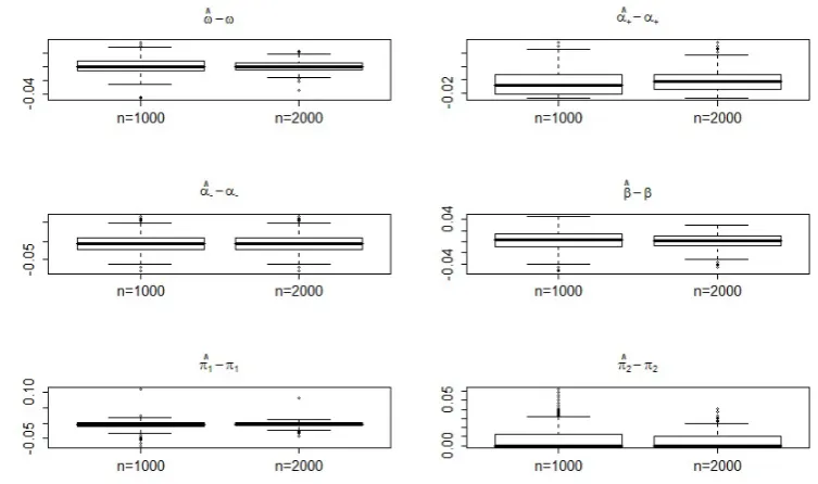
initial values, the first 200 values of each simulation have been eliminated. Figures 1, 2,
3,4display the boxplots of the estimation errors of the QMLE corresponding to the four
noted that the estimators are more accurate when the model is strong (Cases A and B)
than when it is semi-strong (Cases C and D). The boxplots also display more frequent
outliers in the semi-strong case. Also, in accordance with the asymptotic theory, the
distribution of the errors is clearly non Gaussian, especially for the estimation of π02,
when the true value of the parameter stands at the boundary of the parameter space
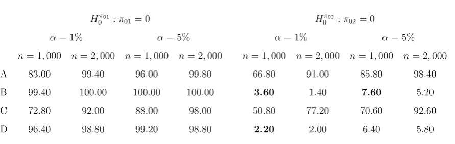
(Cases B and D). Table 1 gives the empirical frequencies of rejection of the hypotheses
π01 = 0 and π02 = 0. The test of the null hypothesis π01 = 0 (which is false in the four
cases) is more powerful in Cases A and B (corresponding to a strong model) than C and
D (corresponding to a semi-strong model). This is not surprising since, as shown by the
boxplots, the semi-strong model is less accurately estimated than the strong one. Less
obviously, the test is slightly more powerful in Cases B and D (when π02 = 0) than in
Cases A and C (when π02 = 0.089). Turning to the test of the null hypothesis π02 = 0
(which is true in Cases B and D), one can see that the type 1 errors are well controlled
when n = 2,000. Indeed, when the nominal level is 5%, the empirical relative frequency
of rejection over the 500 independent replications should vary between 2.2% and 6.6%
with probability of approximately 95%. When the nominal level is 1%, it varies from
0.4% to 2.0% with the same probability. All the relative rejection frequencies displayed
Table 1: Relative frequencies (in %) of rejection of the assumptions that the first and second lagged values of the exogenous variable do not appear in the conditional variance
Hπ01
0 :π01= 0 H0π02 :π02= 0
α= 1% α= 5% α= 1% α= 5%
n= 1,000 n= 2,000 n= 1,000 n= 2,000 n= 1,000 n= 2,000 n= 1,000 n= 2,000
A 83.00 99.40 96.00 99.80 66.80 91.00 85.80 98.40
B 99.40 100.00 100.00 100.00 3.60 1.40 7.60 5.20
C 72.80 92.00 88.00 98.00 50.80 77.20 70.60 92.60
Figure 1: Boxplots of 500 estimation errors for the QMLE of the parameter ϑ0 of a
TARCH-X(1,1) in Case A (strong in the interior) for the two sample sizesn = 1,000 and
n= 2,000.
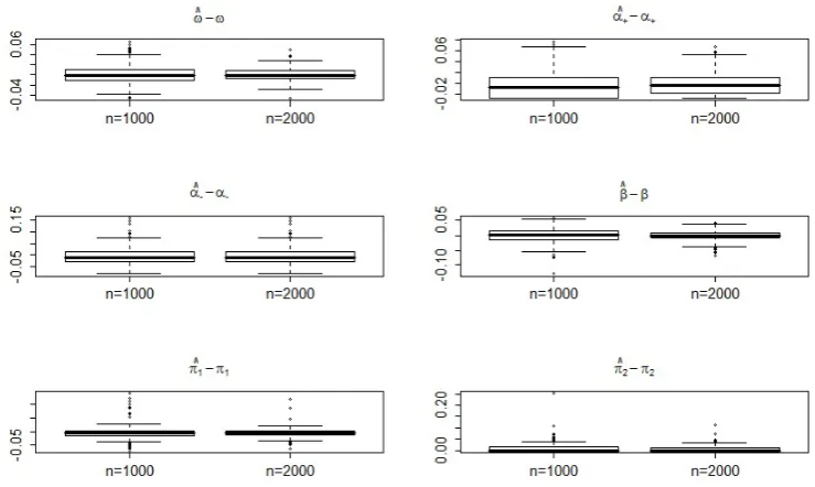
[image:18.595.106.483.421.644.2]Figure 3: As Figure 1 but in Case C (semi-strong in the interior)
[image:19.595.112.482.377.598.2]3.2
SP500 with realized range, volume and other indices
In this section, we built a model which aims to explain the volatility of the daily returns
of the SP500 index by its past values, the realized range, the volume and other stock
returns. The data set has been downloaded from http://finance.yahoo.com/ and
covers the period from January 4, 1985 to August 26, 2011. We considered the series of
the relative range rrt = (hight−lowt)/lowt, where hight and lowt denote respectively
the highest and lowest prices of the day. We also measured the relative volume by the
formula vt =
volt
1 20
P20
i=1volt−i −1
, where volt denotes the daily number of shares traded.
We did not consider directly(volt)as covariate because this series is non stationary. The
indicatorvtcompares the present volume with the averaged volume over the past 20 days,
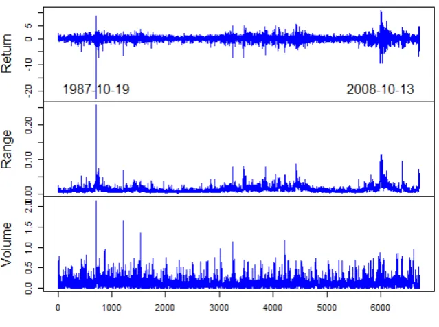
which is a technique used by some traders. Figure 3.2 displays the series of the returns
εt, the ranges rrt and the relative volumes vt, which look stationary. We also added the
returns of the Nikkei,N ikt, and of the FTSE,F tt, as potential explanatory variables for
the SP500 volatility. We fitted APARCH-X(1,1) models with δ ∈ {0.5,1,1.5,2}. The
model with the largest likelihood is obtained for δ= 1, and is given by
εt = htηt
ht= 0.018
(0.006) 0.002+(0.020) 00.000.500ε +
t−1+ 0.110 (0.035) 0.001ε
−
t−1+ 0.879
(0.020) 0.000ht−1+(1.4493) 0.331.002rrt−1
+ 0.061
(0.026) 0.010vt−1+(0.0007) 0.000.500N ik 2
t−1+ 0.000
(0.007) 0.500F t 2
t−1.
Under the estimated value of each coefficient, the estimated standard deviation is given
into brackets, followed by the p-value of the test that the coefficient is equal to zero. One
can see that the range rrt−1 and the volume vt−1 are significant covariates, whereas the returns N ik2
t−1 and F t2t−1 are not. This is in accordance with several empirical studies
showing that the realized range, and to a lesser extent, the volume can help to predict the
volatility (seee.g. Fuertes et al.(2009)). This is also consistent with other studies showing
Figure 5: Return, range and relative volume of the SP500 index from January 4, 1985 to
August 26, 2011 (October 19, 1987 corresponds to the black Monday, and October 13,
3.3
US stocks with realized volatility
The data used in this section come from Section 4.2 ofLaurent et al.(2014)2
and concern
49 large capitalization stocks of american stock exchanges, covering the period from
January 4, 1999 to December 31, 2008 (2,489 trading days). At the end of each trading
dayt, the log-return in percentage εtand the realized volatilityrvt(computed as the sum
of intraday squared 5-minute log-returns) are available.
The first question that we are interested in is whether the realized volatility is useful
to predict the squared returns or not. More precisely, we would like to know how many
lagged values of the realized volatility have to be considered in the volatility equation.
In order to answer this question, we estimated APARCH-X(1,1) models of the form
εt=h1t/δηt
ht =ω+α+(εt+−1)δ+α−(ε −
t−1)δ+βht−1 +π1rvtδ/−21+π2rvtδ/−22,
(22)
with δ ∈ {0.5,1,1.5,2}. The variables rvt−1 and rvt−2 are raised to the power δ/2 in
order to have the same unit of measure forε2
t, the squared volatility h
2/δ
t and the realized
volatilityrvt, regardless ofδ. The selected value ofδ is that which leads to the maximum
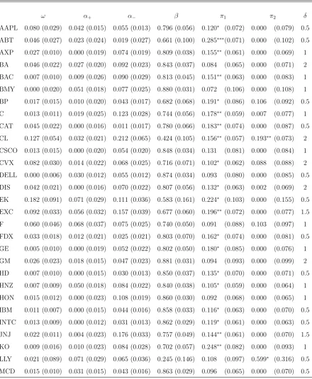
value of the quasi-likelihood. Table 2displays the fitted model on each of the 49 stocks.
For all the estimated models, except 3 over the 49, one observes that α− > α+, which is
in accordance with the leverage effect (i.e. the fact that the volatility tends to increase
more after a negative return than after a positive return of the same magnitude). We
mostly findπ1 significantly non zero and π2 close to zero. From this table, it is clear that
yesterday’s realized volatility often helps in predicting today’s squared return.
Another question that we would like to investigate is whether the realized volatility
is a good proxy of the volatility or not. Of course, the answer depends on what the
precise meaning of "volatility" is. Here, we define the volatility as the best predictor of
the squared return given all the information available Ft−1, consisting in the past returns
and the past realized volatilities. We thus consider the model
εt =h1t/δηt
ht =ω+α+(ε+t−1)δ+α−(ε
−
t−1)δ+βht−1+π0rvtδ/2.
(23)
2
Note that this model is considered for explanatory purposes only, but can not be used
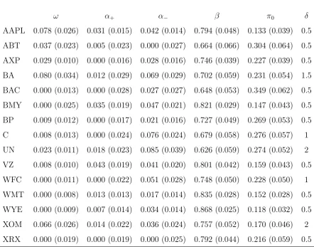
for predicting ε2
t since it involves the unavailable realized volatility at time t. The null
hypothesis that the realized volatility rvt is the best proxy of the volatility ht can be
formally written as
H0 : α+ =α−=β = 0. (24)
No need to use a formal test, the null hypothesis (24) is clearly rejected on all the
estimated models for the 49 stocks (see Table 3), in particular, because the persistent
parameter βb is always highly significant. From this study, we can draw the conclusion
that the realized volatility is far from being an ideal proxy of the actual volatility. It
is thus questionable to compare volatility forecasts with realized volatilities, a practice
which is however becoming common in finance since the celebrated paper of Hansen and
Table 2: APARCH-X(1,1) models (22) fitted by QMLE on daily returns of US stock with two lagged
values of realized volatilities as covariates. The estimated standard deviations are displayed into
paren-theses. For the estimated values ofπ1andπ2, one star (*) means ap-valuep∈[0.01,0.05)for testing the nullity of the coefficient, two stars (**) meansp∈[0.001,0.01), and three stars (***) meansp <0.001.
The last column gives the selected value of the powerδ.
ω α+ α− β π1 π2 δ
AAPL 0.080 (0.029) 0.042 (0.015) 0.055 (0.013) 0.796 (0.056) 0.120∗
(0.072) 0.000 (0.079) 0.5
ABT 0.046 (0.027) 0.023 (0.024) 0.019 (0.027) 0.661 (0.100) 0.285∗∗∗
(0.071) 0.000 (0.102) 0.5
AXP 0.027 (0.010) 0.000 (0.019) 0.074 (0.019) 0.809 (0.038) 0.155∗∗
(0.061) 0.000 (0.069) 1
BA 0.046 (0.022) 0.027 (0.020) 0.092 (0.023) 0.843 (0.037) 0.084 (0.065) 0.000 (0.071) 2
BAC 0.007 (0.010) 0.009 (0.026) 0.090 (0.029) 0.813 (0.045) 0.151∗∗
(0.063) 0.000 (0.083) 1
BMY 0.000 (0.020) 0.051 (0.018) 0.077 (0.025) 0.880 (0.031) 0.072 (0.106) 0.000 (0.108) 1
BP 0.017 (0.015) 0.010 (0.020) 0.043 (0.017) 0.682 (0.068) 0.191∗
(0.086) 0.106 (0.092) 0.5
C 0.013 (0.011) 0.019 (0.025) 0.123 (0.028) 0.744 (0.056) 0.178∗∗
(0.059) 0.007 (0.077) 1
CAT 0.045 (0.022) 0.000 (0.016) 0.011 (0.017) 0.780 (0.066) 0.183∗∗
(0.074) 0.000 (0.087) 0.5
CL 0.127 (0.054) 0.032 (0.021) 0.212 (0.065) 0.424 (0.105) 0.156∗∗
(0.057) 0.193∗∗
(0.073) 2
CSCO 0.013 (0.015) 0.000 (0.020) 0.054 (0.020) 0.848 (0.034) 0.131 (0.081) 0.000 (0.084) 1
CVX 0.082 (0.030) 0.014 (0.022) 0.068 (0.025) 0.716 (0.071) 0.102∗
(0.062) 0.088 (0.088) 2
DELL 0.000 (0.006) 0.030 (0.012) 0.055 (0.012) 0.874 (0.034) 0.093 (0.080) 0.000 (0.085) 0.5
DIS 0.042 (0.021) 0.000 (0.016) 0.070 (0.022) 0.807 (0.056) 0.132∗
(0.063) 0.002 (0.069) 2
EK 0.182 (0.091) 0.071 (0.029) 0.111 (0.036) 0.583 (0.161) 0.224∗
(0.103) 0.000 (0.155) 0.5
EXC 0.092 (0.033) 0.056 (0.032) 0.157 (0.039) 0.677 (0.060) 0.196∗∗
(0.072) 0.000 (0.077) 1.5
F 0.060 (0.046) 0.068 (0.037) 0.075 (0.025) 0.740 (0.050) 0.091 (0.088) 0.103 (0.097) 1
FDX 0.033 (0.018) 0.012 (0.021) 0.025 (0.021) 0.803 (0.070) 0.162∗
(0.074) 0.000 (0.081) 0.5
GE 0.005 (0.010) 0.000 (0.019) 0.052 (0.022) 0.802 (0.050) 0.180∗
(0.085) 0.000 (0.076) 1
GM 0.026 (0.023) 0.018 (0.015) 0.047 (0.023) 0.881 (0.031) 0.094 (0.093) 0.000 (0.099) 2
HD 0.007 (0.010) 0.000 (0.015) 0.030 (0.013) 0.850 (0.037) 0.135∗
(0.070) 0.000 (0.071) 0.5
HNZ 0.007 (0.009) 0.050 (0.018) 0.084 (0.022) 0.840 (0.038) 0.105∗
(0.059) 0.000 (0.064) 1
HON 0.015 (0.012) 0.000 (0.023) 0.108 (0.019) 0.860 (0.030) 0.092 (0.068) 0.000 (0.065) 1
IBM 0.011 (0.007) 0.000 (0.015) 0.044 (0.016) 0.858 (0.033) 0.116∗
(0.063) 0.000 (0.070) 0.5
INTC 0.013 (0.009) 0.000 (0.012) 0.031 (0.013) 0.862 (0.029) 0.119∗
(0.061) 0.000 (0.063) 0.5
JNJ 0.022 (0.011) 0.004 (0.023) 0.176 (0.033) 0.757 (0.049) 0.144∗∗
(0.061) 0.000 (0.070) 1.5
KO 0.009 (0.016) 0.010 (0.023) 0.084 (0.028) 0.702 (0.057) 0.248∗∗
(0.082) 0.000 (0.093) 1
LLY 0.021 (0.089) 0.071 (0.029) 0.065 (0.036) 0.245 (0.146) 0.108 (0.097) 0.599∗
(0.316) 0.5
Table 2: (continued)
ω α+ α− β π1 π2 δ
MMM 0.035 (0.020) 0.011 (0.024) 0.015 (0.024) 0.777 (0.057) 0.181∗
(0.104) 0.000 (0.104) 0.5
MOT 0.011 (0.010) 0.004 (0.014) 0.066 (0.015) 0.888 (0.025) 0.081 (0.067) 0.000 (0.070) 1
MRK 0.022 (0.013) 0.017 (0.017) 0.085 (0.024) 0.904 (0.026) 0.046 (0.073) 0.000 (0.065) 1
MS 0.015 (0.016) 0.011 (0.019) 0.058 (0.022) 0.720 (0.080) 0.251∗∗∗
(0.078) 0.000 (0.102) 0.5
MSFT 0.000 (0.011) 0.046 (0.019) 0.038 (0.015) 0.731 (0.066) 0.237∗∗∗
(0.073) 0.000 (0.100) 0.5
ORCL 0.000 (0.010) 0.001 (0.014) 0.050 (0.016) 0.888 (0.024) 0.095 (0.063) 0.000 (0.065) 1
PEP 0.011 (0.010) 0.042 (0.017) 0.070 (0.021) 0.842 (0.035) 0.084 (0.058) 0.000 (0.066) 2
PFE 0.005 (0.006) 0.014 (0.010) 0.041 (0.010) 0.956 (0.010) 0.014 (0.031) 0.000 (0.029) 2
PG 0.032 (0.021) 0.000 (0.027) 0.134 (0.035) 0.649 (0.074) 0.269∗∗∗
(0.080) 0.000 (0.100) 1
QCOM 0.051 (0.027) 0.029 (0.019) 0.110 (0.024) 0.819 (0.038) 0.116∗
(0.065) 0.000 (0.070) 1.5
SLB 0.116 (0.049) 0.003 (0.017) 0.015 (0.019) 0.827 (0.045) 0.121∗
(0.067) 0.000 (0.073) 2
T 0.008 (0.009) 0.003 (0.013) 0.050 (0.018) 0.881 (0.023) 0.087 (0.055) 0.000 (0.058) 2
TWX 0.000 (0.030) 0.041 (0.028) 0.150 (0.033) 0.564 (0.063) 0.211∗∗
(0.071) 0.166∗
(0.081) 1.5
UN 0.020 (0.010) 0.039 (0.021) 0.108 (0.039) 0.705 (0.064) 0.189∗∗
(0.072) 0.000 (0.078) 2
VZ 0.012 (0.011) 0.050 (0.019) 0.054 (0.020) 0.787 (0.051) 0.162∗∗
(0.063) 0.000 (0.074) 0.5
WFC 0.000 (0.011) 0.020 (0.024) 0.091 (0.029) 0.734 (0.056) 0.120∗
(0.069) 0.100 (0.073) 1
WMT 0.002 (0.006) 0.010 (0.012) 0.047 (0.013) 0.916 (0.016) 0.050 (0.061) 0.000 (0.061) 2
WYE 0.000 (0.008) 0.012 (0.013) 0.042 (0.013) 0.877 (0.029) 0.099 (0.063) 0.005 (0.069) 0.5
XOM 0.073 (0.030) 0.021 (0.021) 0.066 (0.023) 0.742 (0.073) 0.118∗
(0.060) 0.048 (0.085) 2
XRX 0.000 (0.017) 0.010 (0.019) 0.012 (0.020) 0.828 (0.049) 0.170∗∗
Table 3: "Unusable" APARCH-X(1,1) model (23) with contemporaneous realized volatility as covariate (extract).
ω α+ α− β π0 δ
AAPL 0.078 (0.026) 0.031 (0.015) 0.042 (0.014) 0.794 (0.048) 0.133 (0.039) 0.5
ABT 0.037 (0.023) 0.005 (0.023) 0.000 (0.027) 0.664 (0.066) 0.304 (0.064) 0.5
AXP 0.029 (0.010) 0.000 (0.016) 0.028 (0.016) 0.746 (0.039) 0.227 (0.039) 0.5
BA 0.080 (0.034) 0.012 (0.029) 0.069 (0.029) 0.702 (0.059) 0.231 (0.054) 1.5
BAC 0.000 (0.013) 0.000 (0.028) 0.027 (0.027) 0.648 (0.053) 0.349 (0.062) 0.5
BMY 0.000 (0.025) 0.035 (0.019) 0.047 (0.021) 0.821 (0.029) 0.147 (0.043) 0.5
BP 0.009 (0.012) 0.000 (0.017) 0.021 (0.016) 0.727 (0.049) 0.269 (0.053) 0.5
C 0.008 (0.013) 0.000 (0.024) 0.076 (0.024) 0.679 (0.058) 0.276 (0.057) 1
UN 0.023 (0.011) 0.018 (0.023) 0.085 (0.039) 0.626 (0.059) 0.274 (0.052) 2
VZ 0.008 (0.010) 0.043 (0.019) 0.041 (0.020) 0.801 (0.042) 0.159 (0.043) 0.5
WFC 0.000 (0.011) 0.000 (0.022) 0.051 (0.028) 0.748 (0.050) 0.228 (0.050) 1
WMT 0.000 (0.008) 0.013 (0.013) 0.017 (0.014) 0.835 (0.028) 0.152 (0.028) 0.5
WYE 0.000 (0.009) 0.007 (0.014) 0.034 (0.014) 0.868 (0.025) 0.118 (0.032) 0.5
XOM 0.066 (0.026) 0.014 (0.022) 0.036 (0.024) 0.757 (0.052) 0.170 (0.046) 2
4
Conclusion
In this paper, we studied the asymptotic behavior of the QMLE for the versatile class
of the semi-strong PGARCH models augmented with exogenous variables. The main
assumptions on the exogenous variables are the stationarity and non-colinearity with the
other explanatory variables of the volatility. This allows to incorporate some additional
covariates for predicting the volatility of the financial returns, such as the volumes, the
realized ranges, other past squared returns or intraday realized volatilities. Since the true
value of the parameter is not constrained to belong to the interior of the parameter space,
we were able to derive tests for the significance of the exogenous variables. For the
asymp-totic distribution of the QMLE, we investigated four different situations corresponding
to strong or semi-strong models, and to parameters inside or at the boundary of the
pa-rameter space. When the GARCH-X papa-rameter belongs to the interior of the papa-rameter
space, the asymptotic distribution of the QMLE is normal, whereas it is the projection of
a normal distribution on a convex cone when one or several coefficients are equal to zero.
For models with positive coefficients, the asymptotic distribution is obtained under very
mild conditions, in particular, without any moment condition on the observed process.
When the parameter stands at the boundary, moment conditions are required, and the
extra assumptions are stronger for semi-strong than for strong models. Moreover, the
sandwich form of the variance involved in the asymptotic distribution becomes simpler
in the strong case.
The asymptotic theory developed in the paper has been applied to simulations and
real series. Our empirical results are in accordance with numerous applied studies, and
complement them by providing a formal test for the significance of the exogenous
vari-ables. In particular, we generally find useful the volume, the realized range and the
intraday realized volatility for predicting the squares of the financial returns, but none of
5
Proofs and technical lemmas
Proof of Lemma 1. The arguments being quite standard, we just give a sketch of proof (see e.g. Theorem 2.4 in Francq and Zakoïan (2010) for a similar result with a
more detailed proof). Because all the components of C0t and B0t are non-negative, the
components ofYtdefined by (4) are always well defined in[0,+∞]. SinceE|logkB01k|<
∞, by the Cauchy rule, whenγ <0, the components ofYtare shown to be almost surely
finite. The process Yt satisfies (3) and, being a measurable function of (ηt,xt), it is also
stationary and ergodic under A1. The uniqueness of the stationary solution is shown as in the case π0 = 0. For the converse, note that when a (finite) stationary solution exists
for (3), then
lim
k→∞
k Y
i=1
C0,t−i−1
!
B0,t−k = 0 a.s.
Note also that
k Y
i=1
C0,t−i−1
!
B0,t−k≥
k Y
i=1
C0,t−i−1
!
B
where B is obtained by replacing π0 with 0 in B01. Pan et al. (2008) have shown that
k Q
i=1
C0,t−i−1
B →0a.s. entails that γ <0.3
✷
Proof of Lemma 2. The result is known whenπ0 = 0 (see Proposition A.1 in HZ). For notational simplicity, we give the proof for general π0 when p = q = 1. If γ < 0, ht is
then given by (6). Using the elementary inequality(Piui)s≤Piusi for any sequence of
positive numbers ui and any s∈(0,1], and the Cauchy-Schwarz inequality, we obtain
Ehs t ≤
∞
X
k=0
E
k Y
i=1
a(ηt−i)̟t−k−1
!s
= ∞
X
k=0
E
k Y
i=1
as(η
t−i)̟ts−k−1
!
≤
∞
X
k=0
k Y
i=1
Ea2s(ηt−i)E̟t2−sk−1
!1/2
.
By Assumption A1, there exists s > 0 such that E̟2s
t < ∞. Moreover, the fact that
γ =Eloga(ηt)<0and that Ear(ηt)<∞ for some r >0 entails that there exists s >0
such that Ea2s(η
t) <1 (see e.g. Lemma 2.2 in (Francq and Zakoïan, 2010)). It follows
3
Panet al. (2008) employed different assumptions, but a careful examination of their proof and of
Lemma 3.4 inBougerol and Picard (992a) reveals that the assumption that (ηt) is iid, as well as their
that Ehs
t <∞, and thus Eh s/δ
t <∞ for some s >0. By the Cauchy-Schwarz inequality
and A1, we deduce that E|εt|s/2 <∞. ✷
The following lemma is useful to show the identifiability of the parameters under A4.
Lemma 3 Let X be a random variable which takes at least three values and P(X >0)∈
(0,1). If a(X+)δ+b(X−
)δ=c a.s., with a, b, c∈R, then a=b= 0.
Proof. If a = 0 and b 6= 0 then b(X−
)δ =c with probability one. Since P(X > 0)>0,
we must have c = 0. It follows that X−
= 0 a.s. which is in contradiction with the
assumption that P(X >0)<1.
If a 6= 0 and b 6= 0, we obtain X = c
a
1/δ
when X > 0 and X = −c
b
1/δ
when
X <0which is in contradition with assumption that X has at least three values. ✷
Proof of Theorem 1. The consistency can be shown by establishing the following intermediate results:
i) lim
n→∞supϑ∈Θ
Qn(ϑ)−Qen(ϑ)
= 0 a.s. ii) If σt(ϑ) =σt(ϑ0)a.s. then ϑ=ϑ0.
iii) E|ℓt(ϑ)|<∞and if ϑ6=ϑ0, E|ℓt(ϑ)|> E|ℓt(ϑ0)|.
iv) For anyϑ 6=ϑ0, there exists a neighborhood V(ϑ) such that
lim inf
n→∞ ϑ∗∈infV(ϑ)Qn(ϑ
∗
)> Eℓ1(ϑ0) a.s.
The proofs of i), iii) and iv) being essentially the same as when the parameter π is
not present, we only give the proof of ii).
Assume that σt(ϑ) = σt(ϑ0) a.s. By the second part of A5, the polynomials Bϑ(B)
and Bϑ0(B)are invertible. We thus have
Aϑ+(B) Bϑ(B) −
Aϑ0+(B) Bϑ0(B)
ε+t δ
+
Aϑ−(B) Bϑ(B) −
Aϑ0−(B) Bϑ0(B)
ε−t δ
+
π′
B
Bϑ(B)−
π′
0B
Bϑ0(B)
xt= ω0
Bϑ(1) −
ω
Bϑ0(1)
a.s. (25)
If Aϑ+(B)
Bϑ(B) 6
= Aϑ0+(B)
Bϑ0(B)
or Aϑ−(B)
Bϑ(B) 6
= Aϑ0−(B)
Bϑ0(B)
, then there exist c+i0 6= 0 or c
−
i0 6= 0, a
constant e and a sequence of vectors (di)such that
∞
X
i=i0
c+i Bi ε+tδ+ ∞
X
i=i0
c−
i Bi ε
− t δ + ∞ X i=1
Since ε+t δ =σδ t ηt+
δ
and ε−
t δ
=σδ t η
−
t δ
, there exists (a, b)′
∈R2\(0,0) such that
a ηt+−i0
δ
+b η−
t−i0
δ
=ct,i0
where ct,i is a measurable function of {ηt−j, j > i,xt−k, k > 0}. It follows that
La η+t−i0
δ
+b η−t−i0
δ Ft,i0
=L(ct,i0| Ft,i0)
where L(X|Y) denotes the distribution of X given Y. By lemma 3 and A4, we obtain
a=b= 0. Therefore, we have
Aϑ+(B) Bϑ(B)
= Aϑ0+(B)
Bϑ0(B)
and Aϑ−(B)
Bϑ(B)
= Aϑ0−(B)
Bϑ0(B)
(26)
ByA7, we obtainAϑ+(B) =Aϑ0+(B),Aϑ−(B) = Aϑ0−(B)andBϑ(B) =Bϑ0(B). Then
(25) becomes
(π−π0)′xt−1 =ω0−ω,
which entailsπ =π0 and ω=ω0 under A8. Hence, (ii) is proved. ✷
The proof of the asymptotic distribution of the QMLE is split into several technical
lemmas.
Lemma 4 Under the assumptions of Theorem 2,
(i) E
∂ℓt(ϑ0)
∂ϑ
∂ℓt(ϑ0)
∂ϑ′
<∞, E
∂2ℓ
t(ϑ0)
∂ϑ∂ϑ′
<∞.
(ii) J is non-singular and var
∂ℓt(ϑ0)
∂ϑ
=I.
Proof of Lemma 4. First note that the derivatives ofℓt(ϑ) =
ε2
t
σ2
t
+ lnσ2
t are
∂ℓt(ϑ)
∂ϑ =
∂ ∂ϑ
(
ε2
t
(σδ t)
2/δ +
2
δ lnσ
δ t ) = 2 δ
1− ε
2 t σ2 t 1 σδ t ∂σδ t ∂ϑ (27) and ∂ℓ2 t(ϑ)
∂ϑ∂ϑ′ = 2
δ
1− ε
2 t σ2 t 1 σδ t
∂2σδ t
∂ϑ∂ϑ′
+2
δ
δ+ 2
δ ε2 t σ2 t − 1 1 σδ t ∂σδ t ∂ϑ 1 σδ t ∂σδ t
∂ϑ′
. (28)
In Cases A and B (strong model), one can thus prove (i) by showing that
E 1 σδ t ∂σδ t(ϑ0)
∂ϑ 2
and E 1 σδ t
∂2σδ t(ϑ0)
∂ϑ∂ϑ′
<∞. (30)
In Cases C and D (semi-strong model), using the Hölder inequality and E|ηt|4+ν < ∞,
the existence of the first expectation in (i) can be proven by showing that
E 1 σδ t ∂σδ t(ϑ0)
∂ϑ 2+8/ν
<∞. (31)
Thanks toA2, the second expectation of (i) is still obtained by showing (30).
The existence of the moments in (29)–(31) is already known when π0 is absent, (ηt)
is iid andϑ0 belongs to the interior of Θ (see the proof of (i) and (ii) of Theorem 2.2 in
HZ). We now explain the changes in the proof induced by the our particular framework
in the case p=q = 1. The proof can be easily extended to the general case.
Since σδ t =
P∞
j=0βjct,j withct,j =ω+α+ ε +
t−j−1
δ
+α− ε −
t−j−1
δ
+π′
xt−j−1,we have
∂σδ t ∂ω = ∞ X j=0
βj = 1 1−β,
∂σδ t ∂α+ = ∞ X j=0
βj ε+t−j−1
δ , ∂σ δ t ∂α− = ∞ X j=0
βj ε−
t−j−1
δ , ∂σδ t ∂β = ∞ X j=1
jβj−1ct,j,
∂σδ t
∂π = ∞
X
j=0
βjxt−j−1.
Similar expressions hold for the second order derivatives. Noting also that
ω := inf
ϑ∈Θσ
δ
t >0, (32)
under the moment conditions in A11, we have (29) and (30) in Case B, and (30) and (31) in Case D. In Cases A and C, we have
1 σδ t ∂σδ t ∂ω ≤ 1 ω, 1 σδ t ∂σδ t
∂α+ ≤
1 α+ , 1 σδ t ∂σδ t
∂α− ≤ 1 α− , 1 σδ t ∂σδ t
∂πi ≤
1
πi
,
with the notation π = (π1, . . . , πr)′. Using the inequalities
x
1 +x ≤ x
s and (x+y)s ≤
xs+ys, for x, y ≥0and s ∈(0,1], we also have
1 σδ t ∂σδ t ∂β ≤ 1 βωs ∞ X i=1
iβisnωs+αs+ ε+t−i−1
δs
+α−s ε −
t−i−1
δs
+ (π′
xt−i−1)s
o
Note that, for any q ≥1, under the moments assumptions in A1 and A6, we have
ε+t−i−1
δs
q <∞, ε−
t−i−1
δs
q <∞and k(π
′
xt−i−1)skq <∞
for sufficiently small s > 0. It follows that (29) and (31), for any ν > 0, hold true when
all the components of ϑ0 are non-zero. By the same arguments, we can even show the
stronger result that for any s0 >0 there exists a neighborhood V(ϑ0) of ϑ0 included in
Θ such that
E sup
ϑ∈V(ϑ0)
1 σδ t ∂σδ t(ϑ) ∂ϑ s0
<∞ in Cases A and C. (33)
We obtain (30) by similar arguments, which completes the proof of (i) in the two
remain-ing cases A and C.
We now turn to the proof of (ii). Note that the second equality in (11) comes from
(28) and the fact that E(η2
t | Ft−1) = 1. Using (27), we also have var(∂ℓt(ϑ0)/∂ϑ) =I.
It remains to show thatJ is invertible. If it is not the case, then there exists c∈Rdsuch that
c′J c= 4
δ2E
(
1
σ2δ t (ϑ0)
c′∂σ
δ t(ϑ0)
∂ϑ
2)
= 0.
Then a.s., c′∂σ
δ t(ϑ0)
∂ϑ = 0. In view of (10), this implies
c′ 1,(ε+t−1)δ,(ε
−
t−1)δ, . . . ,(ε+t−q)δ,(ε
−
t−q)δ, σtδ−1(ϑ0). . . , σδt−p(ϑ0),xt−1
= 0.
By the arguments used to prove (ii) of Theorem 1, this is impossible with c 6= 0, which
completes the proof of (ii). ✷
Lemma 5 Under the assumptions of Theorem 2, as n → ∞, we have
√ n ∂
∂ϑQen(ϑ0)−
∂
∂ϑQn(ϑ0)
=o(1) a.s., (34)
sup
ϑ∈V(ϑ0)∩Θ
∂2
∂ϑ∂ϑ′Qen(ϑ)−
∂2
∂ϑ∂ϑ′Qn(ϑ)
=o(1) a.s. (35)
for some neighborhood V(ϑ0) of ϑ0,
∂2
∂ϑ∂ϑ′Qen(ϑn)→J in probability when ϑn →ϑ0 in probability, (36)
√
n∂Qn(ϑ0) ∂ϑ
d
Proof of Lemma 5. In this proof, K and ρ denote generic constants whose values can be modified and such thatK >0 and ρ∈(0,1).
By the definition of Qn(ϑ)and Qen(ϑ), (34) and (35) are entailed by
1 √ n n X t=1
∂ℓt(ϑ0)
∂ϑ −
∂ℓet(ϑ0)
∂ϑ
→0 a.s. , (38)
sup
ϑ∈V(ϑ0)∩Θ
∂2ℓ
t(ϑ)
∂ϑ∂ϑ′ −
∂2ℓe
t(ϑ)
∂ϑ∂ϑ′
→0 a.s. (39)
By the arguments used to show (7.60) inFrancq and Zakoïan (2010), we have
∂ℓt(ϑ0)
∂ϑi −
∂eℓt(ϑ0)
∂ϑi
6Kρ
t 1 +Kη2
t 1 + 1 σδ t(ϑ0)
∂σδ t(ϑ0)
∂ϑi
.
UnderA10-A11, we haveEη4
t <∞and (29), and thus the expectation of the right-hand
side of the inequality is bounded by Kρt. It follows that
∞ X t=1
∂ℓt(ϑ0)
∂ϑi −
∂ℓet(ϑ0)
∂ϑi
has a finite expectation, and thus is finite almost surely, which entails (38). The
conver-gence (39) is shown by arguments which follow the scheme of the proof of the last part
of (d) on Page 167 in Francq and Zakoïan (2010).
To establish (36), first note that
P ∂
2
∂ϑ∂ϑ′Qen(ϑn)−J
≥ǫ
≤a1+a2+a3+a4,
where
a1 =P sup
ϑ∈V(ϑ0)∩Θ
∂2
∂ϑ∂ϑ′Qen(ϑ)−
∂2
∂ϑ∂ϑ′Qn(ϑ)
≥ ǫ 3 ! ,
a2 =P sup
ϑ∈V(ϑ0)∩Θ
∂2
∂ϑ∂ϑ′Qn(ϑ)−
∂2
∂ϑ∂ϑ′Qn(ϑ0)
≥ ǫ 3 ! ,
a3 =P
∂2
∂ϑ∂ϑ′Qn(ϑ0)−J
≥ ǫ 3
, a4 =P {ϑn6∈V(ϑ0)}
for any ǫ > 0 and any neighborhood V(ϑ0) of ϑ0. By the assumption that ϑn → ϑ0 in probability, we have a4 → 0 as n → ∞. By (35), for any ǫ > 0 and when V(ϑ0) is
any ǫ > 0. To prove that a2 → 0, it suffices to show that, for all ǫ > 0, there exists a
neighborhood V(ϑ0)of ϑ0 satisfying
lim n→∞ 1 n n X t=1 sup
ϑ∈V(ϑ0)∩Θ
∂2
∂ϑ∂ϑ′ℓt(ϑ)−
∂2
∂ϑ∂ϑ′ℓt(ϑ0)
≤ǫ a.s.
The result follows from the ergodic theorem, the dominated convergence theorem, the
uniform continuity of the second order derivatives of ℓt(ϑ), and by showing that
E sup
ϑ∈V(ϑ0)∩Θ
∂2
∂ϑ∂ϑ′ℓt(ϑ)
<∞ (40)
for some neighborhood V(ϑ0) of ϑ0. Let us begin to prove (40) in Cases B and D by
using A12. In view of (28) and since σt is bounded away from zero, to show (40), it
suffices to establish that
E sup
ϑ∈V(ϑ0)∩Θ
ε2t
∂σδ t
∂ϑ
∂σδ t
∂ϑ′(ϑ)
<∞, Eϑ∈Vsup(ϑ0)∩Θ
ε2t
∂2σδ t
∂ϑ∂ϑ′(ϑ)
<∞. (41)
Now, (10), the second part of A5 and the compactness of Θentail that
∂σδ t
∂ϑi =di,0(ϑ) + ∞
X
k=1
d+i,k(ϑ) ε+t−k
δ
+d−
i,k(ϑ) ε
−
t−k
δ
+π′i,k(ϑ)xt−k,
with
sup
ϑ∈Θ|
di,0(ϑ)| ≤K, sup
ϑ∈Θ
max|d+i,k(ϑ)|,|d−i,k(ϑ)|,kπi,k(ϑ)k ≤Kρk.
The first moment condition in (41) thus follows from the Hölder inequality and A12. The second moment condition is obtained by doing similar developments for the second
order derivatives. We thus have shown (40) in Cases B and D.
To establish (40) in the two other cases, let us first show that, for any s0 > 0, there
exists a neighborhood V(ϑ0)of ϑ0 such thatV(ϑ0)⊂Θand
E sup
ϑ∈V(ϑ0)
σ2
t(ϑ0)
σ2 t(ϑ) s0
<∞ in Cases A and C. (42)
By the arguments used to show (7.51) in Francq and Zakoïan (2010), for all ξ > 0 and
s∈(0,1), there exists a neighborhood V(ϑ0)of ϑ0 such that
sup
ϑ∈V(ϑ0)
σδ t(ϑ0)
σδ
t(ϑ) ≤
K +K
∞
X
j=0
(1 +ξ)jρjsεt−j−1
δs +K ∞ X j=0
(1 +ξ)jρjsxt−j−1
s
Without loss of generality, it can be assumed that2s0/δ≥1. By the Minskowski
inequal-ity, choosing s such that E|ε1|2ss0 <∞ and Ekx1k2ss0/δ < ∞ and choosing for instance
ξ = 1−ρ
s
2ρs , we have
ϑ∈supV(ϑ0)
σ2
t(ϑ0)
σ2 t δ/2 s0 =
ϑ∈supV(ϑ0)
σδ t(ϑ0)
σδ t
2s0/δ ≤K +K
∞
X
j=0
(1 +ξ)jρjs|ε1|δs
2s0/δ
+K
∞
X
j=0
(1 +ξ)jρjskkx1ksk2s0/δ <∞.
Now, in view of (28), A2 and the Hölder inequality entail
E sup
ϑ∈V(ϑ0)
∂2
∂ϑ∂ϑ′ℓt(ϑ)
≤K
1 + supϑ∈V(ϑ0)
σ2
t(ϑ0)
σ2 t(ϑ) 2 (
ϑ∈supV(ϑ0)
1 σδ t
∂2σδ t(ϑ0)
∂ϑ∂ϑ′
2 +
ϑ∈supV(ϑ0)
1 σδ t ∂σδ t(ϑ0)
∂ϑ 2 4 .
Thus, in Cases A and C, (40) comes from (33) and (42), and the analog (33) for second
order derivatives.
By (27), Lemma 4 and A2, the last result, (37), is a consequence of the central limit theorem for square integrable martingale difference of Billingsley (1961). ✷
Proof of Theorem 2. A Taylor expansion ofQen(ϑ)around ϑ0 gives
e
Qn(ϑ)−Qen(ϑ0) =
∂Qn(ϑ0)
∂ϑ′ (ϑ−ϑ0) + 1
2(ϑ−ϑ0) ′
J(ϑ−ϑ0) +Rn(ϑ),
where
Rn(ϑ) = (
∂Qen(ϑ0)
∂ϑ′ −
∂Qn(ϑ0)
∂ϑ′
)
(ϑ−ϑ0) + 1
2(ϑ−ϑ0)
′ ∂2Qen(ϑ
∗ )
∂ϑ∂ϑ′ −J
!
(ϑ−ϑ0),
and ϑ∗ is between ϑ and ϑ0. In view of (34), (35) and (36), as n→ ∞, we have
nRn(ϑn) =oP √
n(ϑn−ϑ0) +oP
nkϑn−ϑ0k2 (43)
when ϑn−ϑ0 =oP(1). Therefore
nRn(ϑn) =oP(1) when √n(ϑn−ϑ0) = OP(1). (44)
Letting
Zn =−J−1√n
∂Qn(ϑ0)
we obtain the following quadratic approximation of the objective function
e
Qn(ϑ)−Qen(ϑ0) =
1 2n
√n(ϑ−ϑ0)−Zn 2
J−
1
2nkZnk
2
J +Rn(ϑ). (45)
Let
ϑZn = arg inf
ϑ∈Θ
√n(ϑ−ϑ0)−Zn J.
Note that
√
n(ϑZn −ϑ0) = Z
C
n for n large enough, (46)
where ZCn denotes the projection of Zn onC. We have
0 ≤ k√n(ϑbn−ϑ0)−Znk2J − k √
n(ϑZn −ϑ0)−Znk 2
J
= 2nnQen(ϑbn)−Qen(ϑZn)
o
+ 2nnRn(ϑZn)−Rn(ϑbn)
o
≤2nnRn(ϑbn)−Rn(ϑZn)
o
,
where the first inequality comes from the definition of ϑZn, the equality from (45), and
the second inequality from the definition of ϑbn. By (46), it follows that
k√n(ϑbn−ϑ0)−Znk2J− kZ
C
n−Znk2J
≤2nnRn(ϑbn)−Rn(ϑZn)
o
. (47)
We now show thatRn(ϑbn)−Rn(ϑZn) = oP(1). By definition ofϑZn and sinceϑ0 ∈Θ, we also have
√n(ϑZn−ϑ0)−Zn
J ≤ kZnkJ.
The Minskowski inequality then entails that
√n(ϑZn −ϑ0)
J ≤√n(ϑZn−ϑ0)−Zn
J +kZnkJ ≤2kZnkJ.
By (37), we have kZnkJ = OP(1), and thus √n(ϑZn −ϑ0) = OP(1). In view of (44), this entailsnRn(ϑZn) =oP(1). By definition of ϑbn and (45), we have
0≤2nQen(ϑ0)−2nQen(ϑbn) = kZnk2J −
√n(ϑbn−ϑ0)−Zn
2
J −2nRn( b
ϑn).
It follows that, by the cr-inequality,
√n(ϑbn−ϑ0)
2J ≤2√n(ϑbn−ϑ0)−Zn
2J +kZnk2J