Munich Personal RePEc Archive
Search and Segregation
Obradovits, Martin
University of Innsbruck
26 July 2017
Online at
https://mpra.ub.uni-muenchen.de/80397/
Search and Segregation
∗
Martin Obradovits
†University of Innsbruck
July 26, 2017
Abstract
Consumers’ willingness to pay for an identical product, e.g. as caused by differ-ences in local income or tastes, may differ greatly across locations. Yet, while a large literature examines consumers’ optimal price and product-search behavior under vari-ous market configurations, the equilibrium effects of such consumer segregation remain unexplored. To this end, I study a stylized model in which two local monopolistic mar-kets differ in size and their consumers’ willingness to pay. After observing their native market’s price, a subset of flexible consumers may travel to the other market at posi-tive cost, hoping for a bargain. I show that as long as the proportion of flexible high-valuation consumers is not too large, active and directed search to the lower-high-valuation market will occur in equilibrium. If the higher-valuation market is relatively large in size, complex mixed-strategy pricing emerges in equilibrium. For regulators, increasing the fraction of flexible consumers tends to be more effective than manipulating search costs.
Keywords:Consumer Search, Segregation, Clustering, Mixed-Strategy Pricing, Asym-metric Market Structure, Active Search
JEL Classification:D43, D83, L11, L13
∗This article was previously circulated under the title “Going to the Discounter: Consumer Search with
Local Market Heterogeneities”. I greatly benefited from helpful feedback from Chris Wilson, Stefan Buehler, Maarten Janssen, Roman Inderst, José Luis Moraga-González, Lan Zhang, as well as seminar participants at the University of Vienna, Goethe University Frankfurt, the SaM Workshop 2015 in Bristol (UK), the 13th An-nual Industrial Organization Conference in Boston, and the 6th Workshop on Consumer Search and Switching Cost in Groningen (NL). Financial support from the University of Innsbruck, Goethe University Frankfurt, the University of Vienna, and the Austrian Science Foundation is gratefully acknowledged.
†Department of Economics, University of Innsbruck, Universitätsstraße 15, 6020 Innsbruck, Austria.
1
Introduction
Consumers’ characteristics often vary considerably across geographically close locations.
For example, many empirical studies document that income tends to be highly segregated in
urban areas—the rich rarely locate door-to-door with the poor.1 Similarly, the local average
income and purchasing power differ greatly between many neighboring countries, such that
cross-border shopping is a widely observed phenomenon.2 Alternatively, even with
identi-cal income, consumers’ tastes may be heterogeneous due to differences in their composition
(young families vs. pensioners, students vs. employees, etc.). But also the usage or
con-sumption of a physically identical good may be more costly or generate less gross utility
for consumers in one location than another, independently of where they purchased it (for
example, because country/state A has different taxation levels than country/state B—cars
come to mind—or because the required infrastructure is less developed in one location than
another).
All of the above examples have two things in common. The first is that consumers in one
local market may have a higher (average) willingness to pay for a given good than consumers
in a nearby, distinct local market. The second is that due to geographical proximity, at least
some consumers may find it optimal to travel from their native market to another if they
perceive its price level to be lower.
Although there is a large theoretical literature dealing with (often heterogeneous)
con-sumers’ optimal search behavior for low prices (or good product matches) and firms’
equi-librium response,3 the specific form of consumer heterogeneity analyzed in this paper
re-mains unexplored: local clustering and segregation of consumers resulting in heterogeneous
demand characteristics across submarkets. The question is then how the presence of such
consumer heterogeneity affects firms’ equilibrium pricing and consumers’ purchasing
be-1See e.g. Bischoff and Reardon (2013) and Florida and Mellander (2015) for recent reports on income
segregation in major U.S. metropolitan areas.
2See e.g. “Swiss Shoppers Storm German Border Towns,” Spiegel Online, 2011. A relatively recent
survey of the vast economic literature on cross-border shopping is given by Leal et al. (2010).
3Seminal papers in the consumer search literature include Diamond (1971) and Stahl (1989) (sequential
havior, given that consumers do not observe prices outside their local market. If consumers
have to incur a strictly positive cost of accessing an outside market, under which
circum-stances would they still be willing to search4? How does this affect firms’ pricing strategy,
and is there scope for beneficial policy intervention?
In order to answer these questions, I study the following stylized setting. There are
two spatially separated markets, each home to an identical local monopolist producing a
homogeneous good. The markets differ in size and their local consumers’ willingness to
pay for the good. Hence, in the absence of a link between the two markets, each firm would
charge the local monopoly price. However, thereisa link between the markets, such that a
subset of “flexible” consumers may travel to the other market at strictly positive cost. The
flexible consumers can be thought of as sophisticated consumers who are aware of the (from
their perspective) outside market’s existence and its characteristics. At the same time, they
do not face prohibitively high costs of accessing the outside market, for example because
they own a car, do not have high opportunity costs of time, or enjoy shopping. In contrast, all
consumers who are not flexible are captive to their local firm. Then, given that the flexible
consumers’ search costs are not prohibitively high, the following main results are obtained.
The first is that if a large fraction of consumers in the high-valuation market is flexible,
paradoxically no search occurs in the unique equilibrium of the game. This is because the
firm in the high-valuation market (henceforth called “H”) finds its local flexible consumers
too important to lose, and optimally charges a sufficiently low price that discourages them
from leaving towards its rival in the low-valuation market (henceforth called “L”). Although
the markets are segregated, there is a strong link between them due to a large fraction of
flexible consumers. Consequently, H’s pricing is fully disciplined by L’s existence, and
search does not take place.
The second major result is that if the fraction of flexible consumers in the high-valuation
market is sufficiently smalland at the same time the high-valuation market is not too large
relative to the low-valuation one, in the unique equilibrium of the game, each firm sets its
4Throughout the paper, I will often speak of “search costs” when referring to consumers’ costs of reaching
price equal to its local consumers’ valuation, and the high-valuation market’s flexible
con-sumers travel to the low-valuation market and purchase there with certainty. L has no
incen-tive to increase its price, as this would drive out its local consumers with a lower willingness
to pay. At the same time, H has no incentive to discourage its local flexible consumers from
searching, as it would have to decrease its price by too much. This situation is reminiscent of
cross-border shopping and other forms of directed travel in which consumers exploit local
price differences. Instead of choosing prices that are low enough to retain all local
con-sumers, firms in a higher-income country may accept that some consumers will purchase
abroad, and tailor their prices towards local consumers who are less mobile—be it due to
opportunity costs, travel costs, lack of information, or other reasons.
The third main result is that, if the high-valuation market is relatively large (and the
proportion of flexible consumers is not too high), a pure-strategy equilibrium fails to exist,
and complex mixed-strategy equilibria with active search emerge. The intuition is as
fol-lows. If H chose the local monopoly price and the flexible high-valuation consumers were
to search, expecting a low price, L would find it optimal to maximally exploit these
con-sumers by (almost) charging the price of its rival, despite driving out its (relatively small
mass of) local consumers. However, this would undermine the high-valuation consumers’
incentive to search in the first place, and even if they searched, this would give firm H a
reason to undercut. This tension can only be resolved by mixed-strategy pricing in which
L probabilistically exploits incoming searchers by pricing above its local consumers’
valu-ation, but then sometimes does not sell at all because it is priced out by its rival. The latter
occurs because with positive probability, H engages in a sale that may beat L’s high-range
prices. Remarkably, if market H is very large compared to L, a novel and second type of
mixed-strategy equilibrium emerges in which H sometimes engages in a deep sale, which
altogether discourages its local flexible consumers from searching. This is necessary to
sufficiently reduce L’s incentive to price above its local consumers’ valuation.
Considering the above findings, my model contributes to the theory of search (for
ho-mogeneous products) by unifying several plausible properties of search markets that are
positive search cost, the famous Diamond (1971) paradox5does not (always) arise: H may
choose prices well below its local monopoly price in equilibrium. This does not only
oc-cur when H finds it optimal to prevent its flexible consumer group from searching due to
competitive pressure by L, but also as an equilibrium response to firm L’s attempt to exploit
incoming searchers. While the former rationale is well-understood in different setups (see
e.g. Reinganum (1979)—compare with the literature discussion below), the latter is, to the
best of my knowledge, novel. The second property is that active search may emerge, as H
may price above its flexible consumers’ reservation price in equilibrium. I argue that this
stems from an interaction of search-cost heterogeneity and spatial heterogeneity in tastes,
and point out that thecombinationof these two is necessary to generate search in the model.
In contrast, standard sequential search models such as Stahl (1989) and Janssen et al. (2005)
induce an endogenous reservation price above which no firm prices in equilibrium,
prevent-ing active search.6 Third, and again to the best of my knowledge, the model is the first
which can simultaneously generate spatial and temporal price dispersion in equilibrium.
The price dispersion is spatial, in the sense of Salop and Stiglitz (1977) and Reinganum
(1979), because L charges prices that are on average lower than H’s. On the other hand,
if no pure-strategy equilibrium exists, the price dispersion is also temporal, in the sense
of e.g. Shilony (1977), Varian (1980) and Rosenthal (1980), because in equilibrium, both
firms sample prices randomly from overlapping supports. Hence, complex sales patterns
arise in which H sometimes engages in promotions which may beat L’s price, or which may
altogether discourage its local flexible consumers from shopping around.
After discussing the different types of equilibria that arise in the baseline model, I turn
to a welfare analysis. I identify two potential sources of welfare loss in the market: wasteful
travel expenditures undertaken by searching high-valuation consumers, and deadweight loss
created by dropout low-valuation consumers. While the former occurs whenever the
frac-tion of flexible high-valuafrac-tion consumers is not too large (otherwise, H fights for its flexible
consumers and the social first-best is achieved), the latter only occurs if a pure-strategy
equi-5Roughly speaking, the Diamond paradox says that if all consumers face positive search costs and search
sequentially, every firm in a symmetric oligopoly must charge the monopoly price in equilibrium.
6Two exceptions are given by Stahl (1996) and Chen and Zhang (2011). In both of these papers,
librium fails to exist. In that case, firm L prices above its local consumers’ valuation with
positive probability in equilibrium. This finding also endogenizes an empirical regularity
that has been widely documented, namely that poorer consumer groups tend to find it more
difficult to access certain product markets (see e.g. Somekh (2012, 2015) and the references
therein). In my model, I show that, if the high-valuation (high-income) market is relatively
large in size, the firm in the low-valuation (low-income) market may consider it optimal to
(probabilistically) exclude its local consumers from purchasing. This is because higher rents
can be extracted from less price sensitive (or more wealthy) shoppers coming from outside.
Regulators aiming to improve market efficiency or consumer surplus may try to
manip-ulate consumers’ search costs or alter the fraction of potentially searching consumers. I
establish that increases or decreases in these variables have no clear-cut effects, such that
even a reduction of search costs or an increase in competition through the fraction of flexible
consumers may backfire. However, one main result is that boosting the fraction of potential
searchers may be less risky, as once a certain threshold is reached, both total social welfare
and consumer surplus will be maximized. This is caused by the competitive pressure that
H faces for its (then large) segment of flexible consumers, which forces it to price
aggres-sively and discourage search. Importantly, this result continues to hold when considering
extensions to downward-sloping individual demand.
Finally, in some markets the assumption that firm L’s price is not observed by H-market
consumers is clearly violated. Moreover, it is a priori unclear how much of the models’
results are driven by unobservable prices outside consumers’ local markets (and their
en-suing search problem), rather than pure transport costs in a perfect-information setting.7
After the main analysis, I thus consider a variation of the baseline model in which the
flex-ible consumers costlessly observe all prices, while they still need to incur strictly positive
travel costs in order to purchase outside of their home market. This has several
advan-tages. First, it allows for a characterization of the resulting pricing equilibria and market
outcomes when all prices are observable, which is arguably more realistic for certain market
environments. Second, it provides a robustness check of the baseline model’s findings with
respect to the described change in information structure. And third, it helps to
disentan-7Note also that comparative statics with respect to search costs may alternatively be interpreted as
gle the different effects of search and transport costs on market outcomes. I find that the
model’s complexity increases significantly if there is a large fraction of flexible consumers:
the baseline model’s pure-strategy equilibrium without search breaks down, and three new
types of mixed-strategy equilibria emerge. At the same time, L-market consumers
unam-biguously benefit relative to the baseline model when there are many flexible consumers,
while total social welfare is reduced. Hence, regulations that improve consumers’ access to
price information may increase consumer surplus at the cost of aggregate welfare.
The remainder of this article is organized as follows. The paragraph below discusses the
related literature in more detail. In Section 2, the model setup is introduced. The different
equilibria of the baseline game are analyzed in Section 3. Section 4 is concerned with
welfare and regulation. An extension to perfect information is provided in Section 5. Section
6 concludes and points out some potential directions for future research. Technical proofs
related to the existence of all characterized equilibria are relegated to Appendix A. Appendix
B establishes uniqueness of the baseline model’s equilibria.
Related Literature This article ties into the literature on price dispersion and consumer
search under asymmetric market configurations. An important early contribution was given
by Narasimhan (1988), who extends Varian’s (1980) classic model of sales (where firms
have symmetric loyal consumer bases, and compete in prices for a perfectly price-sensitive
mass of “shoppers”) to the case of asymmetric shares of loyal consumers across (duopolistic)
firms. However, in contrast to the present work, consumers’ willingness to pay is symmetric,
and (sequential) search is ruled out, as consumers are either perfectly informed about all
prices, or are fully captive to their preferred firm.
Kocas and Kiyak (2006) extend Narasimhan (1988)’s model to oligopoly and allow for
differences in willingness to pay across firms. Similar to Narasimhan, sequential search
is ruled out. Moreover, their model differs from the present contribution because there is
no local clustering of consumers with different valuations: each available product is
val-ued the same by all consumers, although product quality may vary across firms. Instead, I
study a situation in which products are homogeneous, while consumers are segregated and
Reinganum (1979) allows for sequential search, but generates price dispersion through
marginal-cost heterogeneity across a continuum of firms, combined with elastic consumer
demand. In her model, high-cost firms charge consumers’ reservation price, whereas
low-cost firms set their monopoly price. Contrary to the present contribution, consumers are
homogeneous, and no active search arises in equilibrium.
Extending Reinganum’s (1979) model, Benabou (1993) admits heterogeneity in
con-sumers’ search costs on top of firms’ heterogeneity in marginal costs. In his model, low-cost
firms charge their monopoly price, while all others are disciplined by consumers’ (active)
search. There may also be a bunching of prices for certain segments of marginal costs.
Clearly, search is driven by different forces than in the present article, as consumers differ in
their search costs, but not in their valuations. Moreover, there is a continuum of firms, and
mixed-strategy pricing does not occur.
Rajiv et al. (2002) provide a complex marketing model in which differentiated
con-sumers, both with respect to firm loyalty and their valuation for product quality, may search
across vertically differentiated retailers. In their model, search only occurs if at least one
firm advertises its price, and consumers are not segregated. Moreover, the authors’ focus
lies on firms’ equilibrium frequency of advertising prices and their depth of promotional
discounts.
Close in spirit is a recent paper by Astorne-Figari and Yankelevich (2014), who consider
a setup in which duopolistic competitors differ in their number of local (captive) consumers.8
As in my model, these consumers do not directly observe the outside firm’s price, but may
obtain this information at positive cost. In the unique equilibrium, both firms play mixed
strategies, but the price distribution of the firm with the larger mass of local consumers
first-order stochastically dominates that of its rival. The major difference to the present work is
that price dispersion is driven by an atom of shoppers, rather than by a local heterogeneity in
consumers’ willingness to pay. Proper search does not occur in equilibrium, and eliminating
the atom of shoppers leads to the Diamond result. Moreover, the firm with lower average
prices cannot have an incentive to exploit incoming searchers, as non-local consumers with
positive search cost never visit it.
Other related papers that explicitly account for market asymmetries in a search
frame-work are given by Burdett and Smith (2010) and Kuniavsky (2014). In Burdett and Smith
(2010), one dominant firm with a continuum of retail outlets competes with a fringe mass of
atomistic sellers, and consumers employ a noisy search technology in the spirit of Burdett
and Judd (1983). Kuniavsky (2014) extends the standard sequential search model of Stahl
(1989) to allow for heterogeneously sized sellers (where sellers with more outlets have a
higher probability of being sampled first). In both of these papers, price dispersion is driven
by supply-side heterogeneities, rather than market segregation and the resulting differences
in local demand characteristics.
Since all consumers in my model face positive search costs, yet prices are dispersed in
equilibrium, the paper also relates to a small literature on resolving the Diamond paradox
under strictly positive search costs. Examples include Bagwell and Ramey (1992), who
resolve the paradox by consumers making repeat purchases, and Rhodes (2015), who avoids
the problem by considering multi-product retailers.
Finally, since the flexible consumers in my model may find it optimal to exploit local
price differences, this article is also related to a literature on (third-degree) price
discrimina-tion with costly arbitrary, see e.g. Aguirre and Paz Espinosa (2004), Marchand et al. (2000),
Anderson and Ginsburgh (1999), and Wright (1993).
2
Model Setup
Consider the following market. There are two spatially separated local submarketsH(“high
valuation”) andL(“low valuation”) that host one risk-neutral firm each, labeled and indexed
by their locations. The firms compete in prices pH, pL and sell a single homogeneous
product that is offered in their respective market only. The firms’ identical, constant unit
costs are normalized to zero.
A total massα∈(0,1)of consumers live inH, whereas the remaining mass 1−α live
inL. The consumers’ valuations for the homogeneous product are identical within the local
markets. That is, all consumers that live inHhave unit demand up to a maximum valuation
of vH, whereas all consumers that live in L have unit demand up to a lower maximum
In the baseline model, each consumer only observes the price posted by the firm in
her home market. However, some consumers are flexible in the sense that they can travel
to the other market at positive cost, purchasing there if the observed price is lower. For
expositional simplicity, I assume that theL-market consumers are fully captive in the sense
that they will never visit H. Given pL, they either buy directly (if pL ≤vL), or not at all.9
In contrast, some consumers inHhave the possibility to search. Being heterogeneous with
respect to their search behavior, a fraction 1−βofH-consumers is captive as well. Given
pH, they either buy directly (if pH ≤vH), or not at all. On the other hand, a fraction β
ofH-consumers are (potential) searchers: at a travel cost s∈(0,vH−vL),10 they can visit
marketLand return, purchasing there if the observed price is lower. In all of what follows, I
will refer to these potentially searching consumers asflexible H-consumers. Note that in the
model, searching consumers have to return to their home market after observing the other
firm’s price. This setup is both natural and consistent with the usual assumption of free
recallin search models.
The timing of the game is as follows. First, firmsH andLsimultaneously choose their
prices pH and pL, which are then fixed for the rest of the game. Second, each consumer
observes her home market’s price, and all captive consumers buy immediately as long as the
observed price does not exceed their valuation. Third, the massαβof flexibleH-consumers
observe pH, form (potentially probabilistic) beliefs about firmL’s price pL, and optimally
decide whether to searchL, purchase directly atH, or drop out of the market.11 If they do
not visit marketL, they purchase atH, provided that pH ≤vH. If they visit market L, they
9This assumption does not affect any of the results and is only made to streamline the model setup. In
Appendix B, I show that, as long as theL-market consumers’ search costs are bounded away from zero, they will never search in equilibrium, irrespective of their search-cost distribution.
10For s≥v
H−vL, the unique equilibrium of the game is given by the uninteresting case in which H
prices atvH,Lprices atvL, and no consumers search. On the other hand, while the subsequent equilibrium
characterization also fully applies to the case wheres=0, some of the resulting equilibria require the flexible
H-consumers to play the weakly dominated strategy of not always searching initially. And precisely in these cases, there is equilibrium multiplicity, because another equilibrium exists in which the flexibleH-consumers
doalways search initially. In fact, the model extension to perfect information in Section 5 fully characterizes these additional equilibria when settings=0. And conversely, when there is no equilibrium multiplicity, the equilibria of the baseline model coincide with those of the perfect-information framework. Further details are available from the author upon request.
11They might also randomize among some subset of these options in case of indifference, but it turns out
incur the travel cost s, observe L’s price pL, and optimally buy at the cheaper firm (given
that its price does not exceed their valuation).12,13
The solution concept I employ is a “strong” variant of perfect Bayesian equilibrium in
the spirit of Fudenberg and Tirole (1991, Section 6). As is usual, the flexibleH-consumers’
beliefs need to be consistent with firmL’s pricing in equilibrium. Furthermore, the solution
concept imposes some restraints on firms’ signaling abilities. In particular, it entails a
“no-signaling-what-you-do-not-know” property: Even if firmHchooses a price p′H that is never
played in equilibrium, the flexibleH-consumers’ beliefs about firmL’s price are not affected,
since firmH has no more information about firmL’s price than these consumers and hence
cannot signal anything about it. For the present model, this has the same consequences, but
is weaker than assuming passive beliefs.14
Figure 1 provides a graphical summary of the considered market structure. In the next
section, I proceed to solve for the equilibrium of the described game given the parameters
vH,vL,α,β, ands.15
3
Equilibrium Analysis
The game’s different types of equilibria are characterized by the following sequence of
propositions.16
12Note that it is assumed throughout that consumers purchase with certainty whenever they are indifferent
between purchasing or dropping out of the market. Indeed, this is pinned down in any equilibrium where such indifference may arise with positive probability.
13Some further words on tie-breaking. Note that apart from the situation where p
H=vH, the flexibleH
-consumers may be indifferent between some of their available actions under two different circumstances: (i) they may observe a pricepHthat makes them indifferent between purchasing directly atHor searching market L, given their beliefs about firmL’s price, and (ii) after having searched marketL, it may turn out thatpL=pH,
such that they are indifferent between from where to buy. For (i), it is clear that in any equilibrium where this is relevant (i.e., indifference occurs with positive probability), all flexibleH-consumers must buy directly atH. If they did not (such that they purchased atLwith strictly positive probability), firmHwould have a profitable deviation by reducing its price marginally and breaking the indifference. (This argument also relies on the fact that firmHmakes a positive profit in equilibrium, which is evident due to its massα(1−β)of locked-in consumers.) For (ii), it turns out that the tie-breaking rule is not determined in equilibrium, as such ties arise with zero probability in any equilibrium of the game.
14I thank Régis Renault and an anonymous referee for stressing this fact. 15Clearly, eitherv
H,vLorscan be normalized to some arbitrary constant, e.g.,vH=1 (such thatvLands
can be expressed as fractions ofvH). For expositional reasons, I will not do so throughout the paper.
16All existence proofs can be found in Appendix A, while uniqueness of the baseline model’s equilibria is
L H
massα consumers mass 1−αconsumers
valuationvL each valuationvH > vLeach
travel costs∈(0, vH−vL)
pricepL price pH
L’s price unobserved for αβ
αβ
flexibleH-consumers
[image:13.595.108.478.78.221.2]α(1−β) captive consumers
Figure 1: Depiction of the analyzed market.
Proposition 1. Ifβ>β:=1−vLvH+s ∈(0,1), the unique equilibrium of the game is in pure
strategies such that p∗H =vL+s∈(vL,vH), p∗L=vL, and allαβflexible H-consumers pur-chase in H. H’s equilibrium profit is given by Π∗H = (vL+s)α, whereas L’s equilibrium
profit is given byΠ∗L =vL(1−α).
The intuition to Proposition 1 is straightforward: if sufficiently manyH-consumers are
flexible,Hfinds it worthwhile to fight for these consumers and discourage them from
search-ing. The optimal way for H to achieve this is by charging the maximal markup over L’s
price which deters the flexibleH-consumers from searching: p∗L+s. Note moreover that p∗L<vL cannot be part of an equilibrium. If it was,Hwould either find it optimal to charge
p∗L+s<vH(if pL∗is sufficiently close tovL) or the highest possible pricevH (ifp∗L is small). In either case,L could achieve a higher profit by increasing its price a little, as this would
not decrease its demand. Hence, for a large β, the only possible equilibrium is such that
p∗L=vL, p∗H=vL+s, and no search occurs.
Proposition 2. Ifβ<βandα≤α(β):=β(vH−vLvL)+vL∈(αmin,1), whereαmin=v2 vHvL
H−(vL+s)(vH−vL) ∈
(0,1), the unique equilibrium of the game is in pure strategies such that p∗∗H =vH, p∗∗L =vL,
and allαβflexible H-consumers search and purchase in L.17 H’s equilibrium profit is given
byΠ∗∗H =vHα(1−β), whereas L’s equilibrium profit is given byΠ∗∗L =vL(1−α+αβ).
17In the non-generic case whereβ=β, given thatα≤α(β) =α
min, the equilibria of Propositions 1 and 2
coexist (see Figure 2 below for an illustration). This is because forβ=β,His indifferent between discouraging its local flexible consumers from searching (by pricing atvL+s) or maximally exploiting its captive consumers
Intuitively,β<βis simply the converse of the condition in Proposition 1: if sufficiently
few H-consumers are flexible, H would not even find it worthwhile to fight for them ifL
priced at vL deterministically. Instead, H prefers to fully exploit its captive consumers by
pricing atvH, and accepts that all its local flexible consumers will search and buy at the other
firm.
Note that this logic is the key driving force which leads to active search in equilibria
of the game. In typical search models, active search can be generated by taste and product
heterogeneity or search-cost heterogeneity. In my model, it is thecombinationof taste and
search-cost heterogeneity that induces active search. To see this, note that each factor alone
would be insufficient to do so: If the consumers in marketH were homogeneous in search
costs (with common costss>0), firmH would clearly not be willing to let them go in any
equilibrium, so the spatial heterogeneity and clustering of consumers’ valuations would be
unable to induce search. On the other hand, if consumers’ willingness to pay was identical
across submarkets, search-cost heterogeneity would also be insufficient to generate search,
as both firms would simply set their price equal to consumers’ (common) valuation. But
taken together, consumers’ difference in valuations may create a wedge in local monopoly
prices that would lead to a directed outflow of flexible high-valuation consumers, and this
outflow is indeed not prevented by firmH if the fraction of flexibleH-consumers is not too
large.
Althoughβ≤βis necessary to generate the above pure-strategy equilibrium with active
search, it is not sufficient. A further requirement is that the size of market H is not too
large,α≤α(β), which rules out thatLhas a profitable deviation. The logic behind this is as
follows. Clearly, given thatHprices atvH deterministically and does not fight for its flexible
consumers, an expectation of p∗L =vL by the flexible H-consumers would induce them to search. But then, if theH-market is sufficiently important in size (α is large), Lno longer
finds it optimal to charge vL. Namely, rather than to also serve its own local consumers at
this low price,Lwould prefer to exploit the flexible consumers’ beliefs (of findingp∗L =vL
inL) and charge them the highest possible price (vH) for which they do not return toH. This
is the case ifα>α(β).
The outlined incentive to exploit incoming searchers and the tension to resolve it is
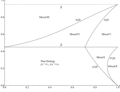
0.6 0.7 0.8 0.9 1.0Α 0.0
0.1 0.2 0.3 0.4 0.5
Β
HILpL*=vL,pH*=vL+s
HIILpL*=vL,pH*=vH
HIIILMixed 1 HIVLMixed 2
Αmin
ΑHΒL
Β
[image:15.595.102.493.84.391.2]ΑHΒL
Figure 2: Equilibrium regions forvH =200,vL=100,s=10.
these equilibria also entail active search by the flexibleH-consumers (at least with positive
probability in the case of Proposition 4). Figure 2 illustrates the different equilibrium regions
in(α,β)-space.
Proposition 3. If β<β and α∈ (α(β),α(β)], where α(β):= vL
(1−β)nvL+vHβ[vH(1−β)−vL]
vH(1−β)−vL−βs
o ∈
(α(β),1),18 the unique equilibrium of the game is in mixed strategies such that19
• H samples prices continuously from the interval [p,vH), where p = vL(1−αβα+αβ) ∈
(vL,vH), following the CDF FH(pH) =1−1−ααβ+αβ
vL pH
. Moreover, H prices at vH
with probability qH∗ := vL(1vHαβ−α+αβ) ∈(0,1).
• L prices at vL with probability q∗L := 1β −vLvHα(1−(α1−+βαβ)) ∈(0,1). Moreover, L
sam-ples prices continuously from the interval [p,vH) following the CDF FL(pL) = 1β−
1−β β
vH pL
.
18Whileα(β)always falls in this range (withα(0) =1 andα(β) =α(β) =α
min), it can be non-monotonic
inβfor certain combinations ofvH,vLands.
19Note that unlike the case whereβ=β, there is no multiplicity of equilibria forα=α(β). This is because
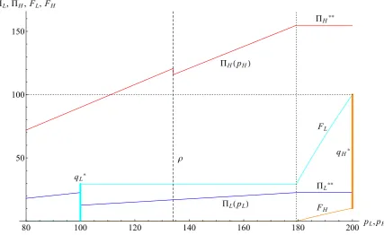
80 100 120 140 160 180 200 pL,pH 50
100 150
PL,PH,FL,FH
PH**
PHHpHL
PL**
PLHpLL
qL*
qH*
FH
FL
[image:16.595.84.512.81.343.2]Ρ
Figure 3: Expected firm profits and equilibrium CDFs for vH =200, vL = 100, s =10, α=0.9, β=0.14. The vertical axis can be interpreted both as monetary units (forΠL(pL) andΠH(pH)) and percentage points (forq∗L,qH∗,FL(.),FH(.)).
• As p>ρ, where the flexible H-consumers’ reservation priceρsolves q∗L(ρ−vL) =s,
all αβ flexible H-consumers search initially. However, they return with probability
1−FL(pH), as in those cases L charges a higher price than H.
• As in the case of Proposition 2, H’s equilibrium profit is given by Π∗∗H, whereas L’s
equilibrium profit is given byΠ∗∗L .
Figure 3 provides a graphical example of an equilibrium of the characterized type.
The intuition to Proposition 3 is as follows. Because theH-market is large compared to
L(α>α(β)), firmLwould no longer find it optimal to chargevLif the flexibleH-consumers
searched (after facingpH=vH and a belief ofpL=vL), as it would strictly prefer to exploit
these consumers’ beliefs by chargingvH instead. However, this cannot be an equilibrium,
because (a) givenpL=vH, the flexibleH-consumers would clearly prefer not to search, and
(b) even if these consumers searched, H would have a profitable deviation by marginally
undercuttingvH (say, by pricing atvH−ε), which would lead all flexible H-consumers to
return toHafter observingpL=vH. Consequently,Lwould also have a profitable deviation
mixed-strategy equilibrium characterized in the proposition: bothLandHprice at their local
consumers’ valuation with positive probability mass, but they also “fight” for the flexibleH
-consumers in those cases whereLprices abovevL.20 In some sense, in order to mitigateL’s
incentive to always exploit the searchers,Halters its strategy in such a way that it becomes
harder forLto sell to the searchingH-consumers if it prices above vL. H achieves this by
spreading positive probability mass on some interval belowvH, implying thatLis indifferent
between choosingvL or any price larger thanvL that lies in that interval.
Since firmLcharges prices higher thanvL with positive probability in equilibrium, this
implies that low-valuation consumers are excluded from buying probabilistically. Hence, the
characterized equilibrium is in line with the empirical finding that low-income consumers
tend to suffer from poor access to certain product markets, as discussed in the introduction.
This continues to hold for the last type of equilibrium to be characterized below.
Proposition 4. Ifβ<βandα∈(α(β),1), the unique equilibrium of the game is in mixed
strategies such that21
• H prices at the flexible H-consumers’ reservation priceρ∗:=vH(1−β)with
proba-bility q∗H,ρ:=1−1αβ−α[vLvH[(vH1−(1β−)−βvL)−]vL2+−vLβsβs]
∈(0,1). Moreover, H samples prices
con-tinuously from [p,vH), where p= vH(vH1−(β1−)[βvH)−(1vL−−β)βs−vL] ∈(ρ∗,vH), following the CDF
FH(pH) =1−q∗H,vH
vH pH
=1−1αβ−α([1vH−(β1)−vLβ[vH)−(vL1−]2β+)vLβs−vL]
vH
pH. Finally, H prices at
vH with probability q∗H,vH:=
1−α αβ
(1−β)vL[vH(1−β)−vL] [vH(1−β)−vL]2+vLβs
∈(0,1).
• L prices at vLwith probability q∗L,vL:= s
vH(1−β)−vL ∈(0,1). Moreover, L samples prices continuously from[p,vH)following the CDF FL(pL) = 1β−1−ββ
vH pL
.
• As H prices at the flexible H-consumers’ reservation priceρ∗with positive probability
q∗H,ρ, these consumers will only search if H prices at or above p>ρ∗, which happens
20The technical reason why a pure-strategy equilibrium may break down is that there may be discontinuities
in firms’ best response functions. For example, ifβ<βandα>α(β), firmL’s best response topH>vLand
(for simplicity) a strategy of always searching by the flexibleH-consumers is p∗L=vL for pH≤vL(1−αβα+αβ)
andp∗L=pH−εfor largerpH. Similarly, firmH’s best response topL≤vHand a strategy of always searching
by the flexibleH-consumers is p∗H =vH for pL≤vH(1−β)andp∗H =pL−εfor higher pL. Due to these
discontinuities, no pure-strategy equilibrium exists in the parameter region in question.
21Note again that unlike the case whereβ=β, there is no multiplicity of equilibria forα=α(β). This is
because the equilibria of Propositions 3 and 4 coincide forα→α(β), as can easily be verified. On the other hand, the equilibria of Propositions 1 and 4 coexist ifβ=βandα>α(β) =αmin(see Figure 2 above for an
illustration). As in the case where Propositions 1 and 2 coexist (ifβ=βandα≤αmin),Lmakes a strictly
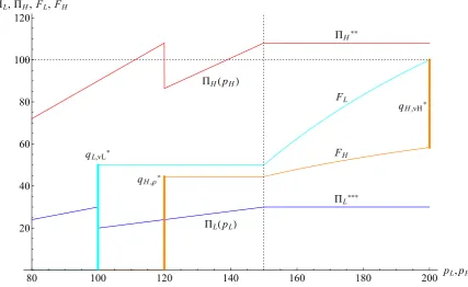
80 100 120 140 160 180 200 pL,pH 20
40 60 80 100 120
PL,PH,FL,FH
PH**
PHHpHL
PLHpLL
PL***
qL,vL*
qH,Ρ*
qH,vH*
FL
[image:18.595.84.512.81.343.2]FH
Figure 4: Expected firm profits and equilibrium CDFs for vH =200, vL = 100, s =10, α=0.9, β=0.4. The vertical axis can be interpreted both as monetary units (forΠL(pL) andΠH(pH)) and percentage points (forqL∗,vL,q∗H,ρ,q
∗
H,vH,FL(.),FH(.)).
with probability1−q∗H,ρ. However, given that H prices at pH ∈[p,vH), they return with probability1−FL(pH), as in those cases L charges a higher price than H.
• H’s equilibrium profit is given by Π∗∗H, whereas L’s equilibrium profit is given by
Π∗∗∗L := (1−α)(1−β)vHvL[vH(1−β)−vL]
[vH(1−β)−vL]2+vLβs .
Again, Figure 4 depicts a graphical example of an equilibrium of the characterized type.
The intuition to Proposition 4 is similar to that of Proposition 3. The crucial difference
is that for a very largeα, theH-market is so important relative toLthat firmLwould always
want to price above its local consumers’ valuation if the flexibleH-consumers searched with
certainty. Indeed, note that since firm H can guarantee to make a profit of vHα(1−β)by
pricing at vH, in equilibrium firm H may never price below vH(1−β)(>vL), as it would
make a lower profit thanvHα(1−β)even if it always sold to the flexibleH-consumers. In
turn, if the flexibleH-consumers searched with certainty,Lcould guarantee to attract them
by pricing at vH(1−β)−ε, making a profit arbitrarily close to vH(1−β)αβ. This profit
close to one.22 Hence, for very largeα,Lcan only be made indifferent between chargingvL
or exploiting the searchingH-consumers if the flexible H-consumers do not always search
initially. H achieves this by putting positive probability mass on the flexibleH-consumers’
reservation priceρ∗=vH(1−β), such thatL cannot even be certain to exploit the flexible H-consumers if it prices at p, the lowest price in its pricing range abovevL.
Note that the equilibrium of Proposition 4, particularly the pricing strategy of firmH,
is consistent with empirical evidence that retail price distributions tend to be bimodal, with
prices fluctuating between a “regular” high price and a low “sales” price, and little mass
between (see Hosken and Reiffen (2004), Pesendorfer (2002)). The present model provides
a complementary explanation to that of Garcia et al. (2015), who generate a two-point price
distribution by introducing costly retailer search for manufacturers’ offers.
4
Welfare and Regulation
In this section, I first pin down the expressions for total social welfare and consumer surplus
that arise in the different equilibrium regions of the model. I proceed to argue which
pa-rameters may be potential targets for policy intervention, and discuss how changes in these
parameters affect total and consumer welfare. Finally, I briefly consider what would happen
if demand was price elastic.
Welfare. Since the consumers have inelastic demand up to a maximum valuation of vH
in H (where a total mass α of consumers reside) and up to vL in L (where the remaining
1−αconsumers reside), it is obvious that the maximal surplus which can be achieved in the
whole market is given by
W :=αvH+ (1−α)vL. (1)
Considering the different equilibria which were outlined in Section 3, there are two
pos-sible sources of welfare loss in the market. First, wasteful travel expenditures to the extent of
22Precisely, this is true forα> vL
(1−β)(vL+vHβ)∈(α(β),1). Although this value is close toα(β)for smallβ (e.g., 0.9084 vs. 0.9045 forvH=200,vL=100,s=10,β=0.14), there is always a non-empty range ofα’s
αβscan be incurred if theαβflexibleH-consumers search. And second, theL-market
sur-plus of(1−α)vL is lost in those cases whereLprices abovevL, as this leads allL-consumers
to drop out of the market. The following proposition then follows straightforwardly from
Propositions 1 to 4.
Proposition 5. The expected total welfare in the market is given by23
W :=
αvH+ (1−α)vL ifβ>β
αvH−αβs+ (1−α)vL ifβ<βandα≤α(β)
αvH−αβs+q∗L(1−α)vL ifβ<βandα∈(α(β),α(β)]
αvH−(1−q∗H,ρ)αβs+q
∗
L,vL(1−α)vL ifβ<βandα∈(α(β),1).
(2)
As consumers’ demand is inelastic, the aggregate expected consumer surplus for each
parameter region can easily be calculated asCS=W−Π[H∗]−Π[L∗], whereΠ[i∗]denotes the
equilibrium profit of firm i∈ {H,L} in the respective parameter region. Clearly, with
in-elastic demand,L-market consumers never make any positive surplus, as firmLnever prices
belowvLin equilibrium.
Proposition 6. The aggregate expected consumer welfare (derived exclusively by H-market
consumers) is given by24,25
CS:=
α(vH−vL−s) ifβ>β
αβ(vH−vL−s) ifβ<βandα≤α(β)
αβ(vH−vL−s)−(1−q∗L)(1−α)vL ifβ<βandα∈(α(β),α(β)]
αβ(vH−vL−s)−(1−q∗L,vL)(1−α)vL
+ q∗H,ραβ(vL+s)
ifβ<βandα∈(α(β),1).
(3)
23Ifβ=β, the expected total welfare depends on which equilibrium is played. It isαv
H+ (1−α)vLifH
playsvL+s, whereas it isαvH−αβs+ (1−α)vL ifHplaysvH (forα≤α(β)), or αvH−(1−q∗H,ρ)αβs+ q∗L,vL(1−α)vLifHplays its (mixed) equilibrium strategy of Proposition 4 (forα>α(β) =α(β)).
24Again, ifβ=β, the equilibrium consumer welfare depends on which equilibrium is played. See footnote
23 above for details.
25In order to obtain the expression for the last case, note thatΠ∗∗∗
Comparative Statics and Regulation. The analyzed model is governed by five
param-eters: Consumers’ maximal willingness to pay in the high and low-valuation market (vH
andvL), the distribution of consumers across markets (α), the search cost of flexible
high-valuation consumers (s), and the share of flexible consumers in the high-valuation market
(β). Note however that the first three of these are rather deep structural parameters that
can-not easily be targeted by policymakers. For example, if the model is used to describe firms’
equilibrium pricing and consumers’ shopping patterns across the neighborhoods of a city,
neither the composition of consumers, nor their different willingness to pay (e.g., as caused
by differences in average income or preferences) can easily be manipulated.
On the other hand, both the search friction of consumers traveling across spatially
sep-arated submarkets (s), as well as the fraction of (flexible) consumers that are aware of this
opportunity and do not find it prohibitively costly to do so (β), may potentially be influenced
by policy.26 For instance, in order to decrease s, the local administration could build new
roads or walkways, improve the public transportation system, or provide amenities such as
parking spaces, public toilets, and temporary childcare facilities. Of course,smay also be
increased through opposing measures.27 Likewise, the fraction of flexible (high-valuation)
consumersβmay be increased by an informational campaign that educates consumers about
the possibility and attractiveness of purchasing in an outside market (with on average lower
prices), infrastructural measures such as the connection of formerly remote areas, or
invest-ment in services like a shuttle-bus line for consumers without cars.
While policy-relevant, analyzing the impact of changes in sorβon total social welfare
and consumer surplus turns out to be a complex task. First, since four different equilibrium
regions arise in the model, changes in s and β may lead to transitions across equilibrium
regions, which, in turn, may have conflicting comparative statics. For example, while total
social welfare is maximal and independent ofsin region I (where no search takes place), it
26Note that bothsandβprovide information about the high-valuation consumers’ search cost distribution.
Indeed, the present model has an identical outcome to the model variation where a fractionβof high-valuation consumers has a search cost ofs, while all remaining high-valuation consumers have search costs that exceed
vH−vL. In a more general model allowing for an arbitrary search-cost distribution, policy-induced shifts of
this distribution could be analyzed.
27As one referee put it, a regulator may want to build a really tall wall between markets in order to
strictly decreases insin regions II and III, while it can be shown that it strictly increases ins
in region IV.28At the same time, consumer surplus strictly decreases insfor regions I to III,
while it strictly increases insfor region IV.29 Second, even within equilibrium regions, the
comparative statics of social welfare and consumer surplus may not be monotone. Precisely,
an increase inβhas an ambiguous effect on social welfare in region III,30while its effect on
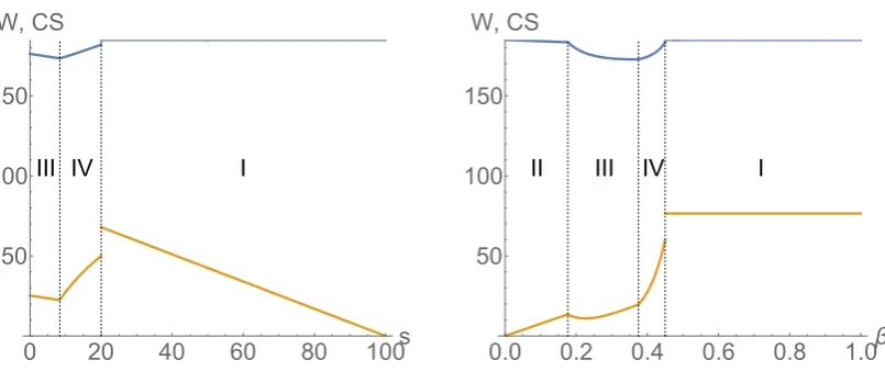
consumer surplus is ambiguous in both regions III and IV.31An example of the comparative
statics of total social welfare and consumer surplus with respect tos and βis provided in
Figure 5.
Although it is thus apparent that no clear-cut comparative statics with respect to sand
β can be provided, some policy recommendation can still be given. Namely, it turns out
that for all parameter values, there is a critical s′ and β′ such that for all s≥s′ (keeping βfixed), or for all β≥β′ (keepings fixed), total social welfare is maximized. Moreover,
consumer surplus is maximized for a single value ofsin this range, namely the lower bound
s=s′, whereas it is maximized for allβ≥β′. These findings are highlighted in the following proposition.32
28That total social welfare strictly decreases insin regions II and III follows from the fact that the flexible
H-consumers always search initially in the corresponding equilibria (creating a wasteful search friction of
αβs), while firmL’s probability of samplingvL (such that no deadweight loss is created) is independent of s. In region IV, an increase insincreases both firmL’s equilibrium frequency of chargingvL and firmH’s
equilibrium frequency of charging the flexibleH-consumers’ reservation priceρ(such that no wasteful search friction is incurred). It can be shown that the welfare gains induced by this always dominate the welfare loss stemming from higher search costs in those cases where firmHprices aboveρ. A proof is available from the author upon request.
29The latter effect is surprising and stems from the fact that both firmL’s equilibrium probability of charging
vL and firmH’s equilibrium probability of chargingρ(the lowest price in its support) strictly increase insin
the relevant region (see also the previous footnote related to social welfare). This is always sufficient to offset the higher travel cost incurred by searching high-valuation consumers (in those cases whereH prices above
ρ). A proof is once again available from the author upon request.
30The intuition for this is that countervailing effects are at play. Since all flexible H-consumers search
initially in region III, an increase in their absolute number throughβ leads to an unambiguous increase in the wasteful search frictionαβsthat is incurred. On the other hand, there are parameter constellations within region III under which firmL’s equilibrium probability of samplingvL increases in β, which reduces the
(expected) deadweight loss that stems from dropout low-valuation consumers. For some of these parameter constellations, the latter positive effect on welfare dominates.
31Again, these surprising results are caused by firms’ equilibrium responses. In region III (IV), consumer
welfare may decline because an increase inβ may lead firmL(H) to reduce its equilibrium probability of chargingvL(ρ).
32For the proposition, it is assumed that equilibrium type I (without search) is played whenever β=β
(which is the unique equilibrium for anyβ>β). The statement for social welfare is obvious (region I without any welfare losses is reached if and only ifs≥s′ orβ≥β′). The statement for consumer surplus follows because allH-consumers are able to buy at the lowest possible effective pricevL+s(firmLmay never price belowvL in any equilibrium) if and only if equilibrium type I is played. Ifsis allowed to vary, this price is
0 20 40 60 80 100s 50
100 150
W, CS
III IV I
0.0 0.2 0.4 0.6 0.8 1.0β
50 100 150
W, CS
[image:23.595.98.501.81.250.2]II III IV I
Figure 5: Expected total social welfare (blue) and consumer surplus (orange) as functions ofs(left panel) andβ(right panel). The parameters used arevH=200,vL=100,α=0.85,
as well asβ=0.4 (left panel) and s=10 (right panel). The different equilibrium regions
that are reached are separated by dotted lines.
Proposition 7. For any combination of parameters vH, vL, α and β, total social welfare
is maximized if and only if s≥s′ :=max{vH(1−β)−vL,0}, while consumer surplus is
maximized if and only if s=s′. Likewise, for any combination of parameters vH, vL,αand s, both total social welfare and consumer surplus are maximized if and only ifβ≥β′:=β.
A regulator that aims to maximize total social welfare and consumer surplus (which
seems sensible, given that both objectives can be achieved simultaneously) thus faces two
options. First, it may try to find the “sweet spot” for the search cost s such that it is just
high enough that H finds it optimal to fight for its local flexible consumers by pricing at
vL+s(and not chargingvH or sampling prices from[p,vH], withp>vL+s), but not higher
than that. If vH(1−β)−vL ≤0, then this is the case even fors=0, such that a regulator
that is (also) concerned for consumer surplus should aim to reduce consumers’ search costs
as much as possible. If instead vH(1−β)−vL >0, the optimals is positive, and hence a
regulator may even have an incentive to artificially increase s (making the outside market
less accessible, levying taxes, etc.) if s is low initially. In reality, a regulator may find it
hard to justify such measures (which, after all, may have severe negative consequences for
society that are not captured in the model), and even in the context of the model, it runs a risk
of harming consumers (compare with Figure 5, left panel). Hence, it seems that influencing
competitive pressure (region I), then reducingsmay increase consumer welfare, but there is
a risk that firms in a high-valuation market may respond by increasing their prices in order
to exploit locked-in consumers—which, at the same time, induces wasteful search frictions.
On the other hand, if there is search initially, increasingsmay restore the first-best, but this
may also harm consumers when done incorrectly, face resistance from the population, and
have adverse consequences that are not part of this analysis.
The second option a regulator may have is to raise the fraction of flexible high-valuation
consumersβ. Although marginal increases inβmay still have a (moderately) negative effect
on welfare and consumer surplus (compare with Figure 5, right panel), there is no longer a
danger of “overshooting”: Once a certain threshold is surpassed (β≥β), full market
effi-ciency is restored, and consumers’ surplus is maximized. The intuition is that a sufficiently
large fraction of non-loyal high-valuation consumers is able to fully discipline the
behav-ior of the local incumbent, even though no search takes place. This is because, by these
consumers’ (correct) expectations of finding pL =vL in marketL, firm H cannot afford to
charge a higher price thanvL+s, as this would turn away a sizable chunk of its demand. In
other words, efficiency is restored precisely becauseH faces a threat of search by a large
fraction of its local consumers, to which it responds by pricing aggressively (and thus, the
threat does not materialize).
Note that there can be circumstances where increasing the fraction β of potentially
searching consumers is not very costly: Indeed, it may suffice to inform (a larger fraction of)
the population that searching is a viable strategy. On the other hand, especially reductions in
scould require infrastructural measures that are prohibitively expensive. Thus, promoting
thepossibilityof search may often be more beneficial than actually inducing search through
a physical reduction in search costs.
Downward Sloping Demand The showcased model focuses on inelastic consumer
de-mand in order to build intuition and keep the analysis tractable. Of course, this comes at the
cost of realism, such that it would be desirable to allow for (a) downward-sloping individual
demand and/or (b) heterogeneous consumer valuations within submarkets. While providing
a full equilibrium analysis is challenging for both of these variations (and lies somewhat
in the baseline model:33 If the fraction of flexible consumers in the market with a higher
local monopoly price is sufficiently large, there will be no search in equilibrium, as the
local incumbent finds it optimal to discourage these consumers from searching by pricing
aggressively. In contrast, the firm in the neighboring low-valuation market charges the local
monopoly price. In the setup with downward-sloping individual demand, it can be shown
that this equilibrium is constrained-efficient, as no wasteful search frictions are incurred,
and deadweight loss is minimized. Indeed, increasing β should generally be (even) more
desirable under elastic demand, as giving a larger fraction of consumers access to low prices
will tend to reduce deadweight loss.
5
Perfect Information Setting
In contrast to the specification of the main model, consumers may sometimes be
well-informed about the prices charged by firms in a distinct regional market. For example, a
consumer considering cross-border shopping for some expensive good (e.g. a new car) will
likely try to obtain price quotesbefore traveling to the outside market.34 Moreover, as
mo-tivated in the introduction, it seems worthwhile to check the baseline model’s robustness
with respect to changes in the information structure, and to contrast the different effects of
search costs (in the sense of information-acquisition costs) and pure travel costs on market
outcomes. While an exhaustive comparison between all variables of interest (equilibrium
pricing strategies, firm profits, consumer surplus and total social welfare) across the
differ-ent model setups would be beyond the scope of this paper, some selected key differences
will be highlighted.
To this end, I consider a variation of the main model in which flexible H-market
con-sumers can perfectly observe the price posted by firmL. However, they still have to incur
a travel costsin order to access marketL. Hence, in the corresponding perfect-information
framework, flexibleH-consumers find it optimal to purchase fromLwhenever pL <pH−s
(≤vH−s). All other market parameters (α, β, vH andvL) keep the same interpretation as
in the main model. Importantly, in order to facilitate a comparison with the baseline setup,
33Details are available from the author upon request.
34Clearly, the rise of price-comparison platforms on the internet, as well as the tendency of many firms to
I still assume that all L-market consumers are fully locked in to their local firm, and that
s<vH−vL.
Note that in this adaptation, it still holds that for a small fraction β of flexible H
-consumers, firmH would not even be willing to fight for these consumers if firmLcharged
vL deterministically. The corresponding critical value ofβ is again given byβ=1−vLvH+s.
Hence, forβ≤β, one might expect that similar types of equilibria emerge as in the baseline
model. However, forβ>β, firmH finds it no longer sufficient to price atvL+sin order to
optimally discourage its local flexible consumers from searching. In contrast to the baseline
model, where firmLcould not credibly convey that it may ever set a price belowvL, this is
now clearly possible by simply setting an arbitrary price pL<vL. As it turns out, this
varia-tion introduces substantial addivaria-tional complexity when the fracvaria-tion of flexibleH-consumers
βis large. In what follows, I will separately consider the casesβ≤βandβ>β.
Proposition 8. Suppose that the flexible H-consumers observe pL, and thatβ≤β. Then
there exist three types of pricing equilibria.
(Pure) If α is small, α ≤α′(β):= β(vH−vLvL)+vL−βs, where α′(β)∈(α(β),1), there is a
pure-strategy equilibrium in which p∗H=vH, p∗L=vL, and all flexible H-consumers purchase in L. L-market consumers are always served in this equilibrium. Firm H makes a profit of
Π∗∗H, while firm L makes a profit ofΠ∗∗L .
(Mixed I) Ifαis intermediate,α∈(α′(β),α′(β)], whereα′(β):= vL(1−β)+βvL[vH(1−β)−s]∈
(α′(β),1), the following constitutes an equilibrium:
• H samples prices continuously from the interval[p
H,vH), where pH =
vL(1−α+αβ)
αβ +
s>vL+s, following the CDF FH(pH) =1−1−ααβ+αβ
vL pH−s
. Moreover, H prices at
vH with probability qH =1−ααβ+αβ
vL vH−s
∈(0,1).
• L prices at vL with probability qL = β1−1−ββ vH vL1−ααβ+αβ+s
!
∈ [0,1). Moreover,
L samples prices continuously from the interval[p
H−s,vH−s) following the CDF FL(pL) =β1−1−ββ
vH pL+s
.
• L-market consumers are only sometimes served in this equilibrium.