Munich Personal RePEc Archive
Making Markowitz’s Portfolio
Optimization Theory Practically Useful
BAI, ZHIDONG and LIU, HUIXIA and WONG,
WING-KEUNG
Northeast Normal University, National University of Singapore, Asia
University
8 October 2016
Making Markowitz’s Portfolio Optimization Theory
Practically Useful
∗
ZHIDONG BAI
KLASMOE and School of Mathematics and Statistics
Northeast Normal University
Department of Statistics and Applied Probability
Risk Management Institute
National University of Singapore
HUIXIA LIU
Department of Statistics and Applied Probability
National University of Singapore
WING-KEUNG WONG
†Department of Finance, Asia University, Taiwan
Department of Economics, Lingnan University, Hong Kong
October 8, 2016
∗The authors would also like to show our appreciation to Professor Oliver B. Linton, Professor Dilip
B. Madan, and Professor Harry M. Markowitz for their helpful comments and thank participants at the 2007 International Symposium on Financial Engineering and Risk Management for their valuable comments. The research is partially supported by NSF grant No.10571020 from China and the grant R-155-000–061-112 from Department of Statistics and Applied Probability, National University of Singapore and the grant R-703-000-015-720 from Risk Management Institute, National University of Singapore, Asia University, and Lingnan University.
†Address correspondence to Wing-Keung Wong, Department of Finance, College of Management, Asia
The traditional estimated return for the Markowitz mean-variance optimization has
been demonstrated to seriously depart from its theoretic optimal return. We prove that
this phenomenon is natural and the estimated optimal return is always √γ times larger
than its theoretic counterpart where γ = 1
1−y with y as the ratio of the dimension to
sample size. Thereafter, we develop new bootstrap-corrected estimations for the optimal
return and its asset allocation and prove that these bootstrap-corrected estimates are
proportionally consistent with their theoretic counterparts. Our theoretical results are
further confirmed by our simulations, which show that the essence of the portfolio analysis
problem could be adequately captured by our proposed approach. This greatly enhances
the practical uses of the Markowitz mean-variance optimization procedure.
KEY WORDS: Optimal Portfolio Allocation, Mean-Variance Optimization; Large
1
INTRODUCTION
The pioneer work of Markowitz (1952, 1959) on the mean-variance (MV) portfolio
optimization procedure is the milestone of modern finance theory for optimal portfolio
construction, asset allocation, and investment diversification. In the procedure,
portfo-lio optimizers respond to the uncertainty of an investment by selecting portfoportfo-lios that
maximize profit subject to achieving a specified level of calculated risk or, equivalently,
minimize variance subject to obtaining a predetermined level of expected gain (Markowitz
(1952, 1959, 1991), Merton (1972), Kroll, Levy and Markowitz (1984)).
Despite the fact that the conceptual framework of the classical MV portfolio
optimiza-tion had first been set forth by Markowitz more than half a century ago, and despite the
fact that several procedures for computing the corresponding estimates (see, for example,
Sharpe (1967, 1971), Stone (1973), Elton, Gruber, and Padberg (1976, 1978), Markowitz
and Perold (1981) and Perold (1984)) have produced substantial experimentation in the
investment community for nearly four decades, there have been persistent doubts about
the performance of the estimates. Instead of implementing nonintuitive decisions
dic-tated by portfolio optimizations, it has long been known anecdotally that a number of
experienced investment professionals simply disregard the results or abandon the entire
approach, since many studies (see, for example, Michaud (1989), Canner, Mankiw, and
Weil (1997), Simaan (1997)) have found the MV-optimized portfolios to be unintuitive,
thereby making their estimates do more harm than good. For example, Frankfurter,
Phillips, and Seagle (1971) find that the portfolio selected according to the Markowitz
MV criterion is likely not as effective as an equally weighted portfolio, while Zellner and
Chetty (1965), Brown (1978), Kan and Zhou (2007) show that the Bayesian decision rule
under a diffuse prior outperforms the MV optimization. Michaud (1989) notes that MV
optimization is one of the outstanding puzzles in modern finance and that it has yet to
meet with widespread acceptance by the investment community, particularly as a
practi-cal tool for active equity investment management. He terms this puzzle the “Markowitz
To investigate the reasons why the MV optimization estimate is so far away from its
theoretic counterpart, different studies have produced a range of opinions and
observa-tions. So far, all believe that it is because the “optimal” return is formed by a
combina-tion of returns from an extremely large number of stocks (see, for example, McNamara
(1998)). Jorion (1985), Best and Grauer (1991) and Britten-Jones (1999) suggest the
main difficulty concerns the extreme weights that often arise when constructing sample
efficient portfolios that are extremely sensitive to changes in asset means. Another school
suggests that the estimation of the correlation matrix plays an important role in this
prob-lem. For example, Laloux, Cizeau, Bouchaud, and Potters (1999) find that Markowitz’s
portfolio optimization scheme which is based on a purely historical determination of the
correlation matrix, is not adequate because its lowest eigenvalues dominating the smallest
risk portfolio are dominated by noise.
Many studies have tried to show that the difficulty can be alleviated by using different
approaches. For example, Pafka and Kondor (2004) impose some constraints on the
correlation matrix to capture the essence of the real correlation structure. Although this
is expected to improve the overall performance, it may certainly introduce some biases in
the estimation. In addition, by introducing the notion of ‘factors’ influencing the stock
prices, Sharpe (1964), Cohen and Pogue (1967) and Perold (1984) formulate the single
index model to simplify both the informational and computational complexity of the
general model. Konno and Yamazaki (1991) propose a mean-absolute deviation portfolio
optimization to overcome the difficulties associated with the classical Markowitz model
but Simaan (1997) finds that the estimation errors for both the mean-absolute deviation
portfolio model and the classical Markowitz model are still very severe, especially in small
samples.
Our paper complements the theoretical work of Markowitz by developing a new
bias-corrected estimator to reliably capture the essence of portfolio selection. We will first
explain and thereafter share the theoretical proofs of our discovery about the “Markowitz
and Potters (1999) and others on this issue that the empirical correlation matrix plays
an important role in this problem. We also find that the estimation of the optimal
return is poor due to the poor estimation of the asset allocations.1 When the dimension
of the data is large, by the theory of the large dimensional random matrix, it is well
known that the sample covariance matrix is not an efficient estimator of the population
covariance matrix2. Thus, plugging the sample mean and covariance matrix into the MV
optimization procedure will result in a serious departure of the optimal return estimate
and the corresponding portfolio allocation estimate from their theoretic counterparts when
the number of the assets is large. In the remainder of this paper, this return estimate
will be called the “plug-in” return, and its corresponding estimate for the asset allocation
will be called the “plug-in” allocation.3 We also prove that the plug-in return is always
larger than its theoretical value with a fixed rate depending on the ratio of the dimension
to sample size.4 We call this phenomenon “prediction.” To circumvent this
over-prediction problem, we further propose a new method to reduce this error by incorporating
the idea of bootstrap into the theory of large dimensional random matrix. The principal
consideration of bootstrap is that there is a similar relationship between the biases of the
estimators based on the original sample and the resampled one. By doing this, we obtain a
bootstrap-modified estimate that analytically corrects the over-prediction and drastically
reduces the error. We further theoretically prove that the bootstrap-corrected estimate of
return and its corresponding allocation estimate are proportionally consistent with their
counterpart parameters. Our simulation further confirms the consistency of our proposed
estimates, implying that the essence of the portfolio analysis problem could be adequately
captured by our proposed estimates. Our simulation also shows that our proposed method
improves the estimation accuracy so substantially that its relative efficiency5 could be as
1
We note that A¨ıt Sahalia and Brandt (2001) suggest focusing directly on the optimal portfolio weights first. This could provide an alternative solution to overcome the Markowitz optimization enigma.
2
See, for example, Laloux, Cizeau, Bouchaud, and Potters (1999).
3
See, for example, Zellner and Chetty (1965), Brown (1978) and Kan and Zhou (2007).
4
We note that Maller, Durand, and Lee (2005) also prove the maximum Sharpe ratio is biased upward for its population value.
5
high as 139 times when compared with the traditional “plug-in” estimate for 300 assets
with a sample size of 500. The relative efficiency will be much higher for bigger sample
sizes and larger numbers of assets. Similar results are also obtained for its corresponding
allocation estimate.
2
THEORY
This section studies the theoretic optimal solution for Markowitz’s MV optimization
pro-cedure and introduces the theory of the large dimensional random matrix to explain
the “Markowitz optimization enigma,” which holds that the Markowitz MV optimization
procedure is impractical. In the next section, we invoke a new approach to make the
opti-mization procedure more practically useful. To distinguish the well-known results in the
literature from the ones derived in this paper, all cited results will be calledPropositions
and our derived results will be calledTheorems.
2.1
Optimal Solution
Suppose that there are p-branch assets, S = (s1, ..., sp)T, whose returns are denoted by
r= (r1, ..., rp)T with meanµ= (µ1, ..., µp)T and covariance matrix Σ = (σij). In addition,
we suppose that an investor will invest capitalC on the p-branch assets Ssuch that s/he
wants to allocate her/his investable wealth on the assets but obtain any of the following:
1. to maximize return subject to a given level of risk, or
2. to minimize her/his risk for a given level of expected return.
Since the above two problems are equivalent, we only look for a solution to the first
problem in this paper.6 Without loss of generality, we assumeC ≤1 and her/his
invest-6
Readers may refer to (1) for the formulation of the maximization problem. This problem is equivalent to
σ2
= mincTΣcsubject tocT1≤1 andR≤cTµ. (1a)
ment plan to be c= (c1, ..., cp)T. Hence, we have ∑pj=1cj =C ≤1. Also, the mean and
risk of her/his anticipated return will then be cT
µand cTΣc, respectively. In this paper,
we further assume that short selling is allowed, and hence any component of c could be
negative. Thus, the above maximization problem can be re-formulated as the following
optimization problem:
R= max cTµ, subject to cT1 ≤1 and cTΣc≤σ02 (1)
wherelrepresents the p-dimensional vector of ones andσ2
0 is a given risk level.7 We callR
satisfying (1) the optimal return and the solutionc to the maximization theoptimal
allocation plan. One could easily extend the separation Theorem (Cass and Stiglitz
(1970)) and the mutual fund theorem (Merton (1972)) to obtain the analytical solution
of (1)8 from the following Proposition:
PROPOSITION 1 For the optimization problem shown in (1), the optimal return,
R, and its corresponding investment plan,c, are obtained as follows:
1. If
1TΣ−1µσ0
√
µTΣ−1µ
<1,
then the optimal return, R, and corresponding investment plan, c, will be
R=σ0
√
µTΣ−1µ
and
c= √ σ0
µTΣ−1µ
Σ−1µ.
2. If
7
We note that in this paper we study the optimal return. However, another direction of research is to study the optimal portfolio variance; see, for example, Pafka and Kondor (2003) and Papp, Pafka, Nowak, and Kondor (2005).
8
1TΣ−1µσ0
√
µTΣ−1µ
>1,
then the optimal return, R, and corresponding investment plan, c, will be
R = 1
TΣ−1
µ
1TΣ−11 +b
(
µTΣ−1µ− (
1TΣ−1µ)2 1TΣ−11
)
,
and
c= Σ
−11
1TΣ−11+b
(
Σ−1µ−
1TΣ−1µ 1TΣ−11Σ
−11
)
where
b =
√
1T ∑−11σ2
0 −1
µTΣ−1µ1TΣ−11−(1TΣ−1µ)2
.
The proof of Proposition 1 can be found from many references in the literature.
REMARK 1 The intuition of the inequalities to distinguish the two cases of the
so-lutions in Proposition 1 can be seen from the following: The maximization is taken in the
intersection of the ellipsoid cTΣc≤σ
0 and the half space cTl≤1 (note that the
intersec-tion is not empty because the point c=0 belongs to both the half space and the ellipsoid).
If the ellipsoid is completely contained in the half space, that is, the ellipsoid does not
intersect with the hyperplane cTl= 1, then the solution is the same as the maximization
problem without the half space restriction. Hence, the solution is then given by the first
case. Otherwise, the maximizer should be on the intersection of the ellipse cTΣc = σ
0
and the hyperplane cTl = 1, since the target function cT
µ is a linear function in c. The
inequality 1TΣ−1µσ0
√
µTΣ−1µ <1 could then be used to test whether the maximizer of c
T
µ is in
the ellipsoid, i.e., whether c= Σ−1µσ0
√
µTΣ−1µ is an inner point of the half space.
The set of efficient feasible portfolios for all possible levels of portfolio risk forms the
MV efficient frontier. We note that in this paper we formulate the p-branch assets for
this optimization problem in which the assets could be common stocks, preferred shares,
to be available for both borrowing and lending and that excess return is calculated by
subtracting the return of this riskless asset from the total return. The return calculated in
this paper could be set as the total return or the excess return. For any given level of risk,
Proposition 1 seems to provide a unique optimal return with its corresponding MV-optimal
investment plan or asset allocation to represent the best investment alternative given the
selected assets. Thus, it seems to provide a solution to Markowitz’s MV optimization
procedure. Nonetheless, one may expect the problem to be straightforward; however, this
is not so, since the estimation of the optimal return and its corresponding investment plan
is a difficult task. This issue will be discussed in the following sections.
2.2
Large Dimensional Random Matrix Theory
The large dimensional random matrix theory (LDRMT) traces back to the development
of quantum mechanics (QM) in the 1940s. Because of its rapid development in theoretic
investigation and its wide application, it has since attracted growing attention in many
areas, such as economics and finance, as well as mathematics and statistics. Wherever
the dimension of data is large, the classical limit theorems are no longer suitable, since
the statistical efficiency will be substantially reduced when they are employed. Hence,
statisticians have to search for alternative approaches in such data analysis, and thus,
the LDRMT is found to be useful. A major concern of the LDRMT is to investigate the
limiting spectrum properties of random matrices where the dimension increases
propor-tionally with the sample size. This turns out to be a powerful tool in dealing with large
dimensional data analysis.
We utilize the LDRMT (Bai, et al., 2011) to study MV optimization by analyzing
the corresponding high dimensional data. In the analysis, an estimation of the sample
covariance matrix plays an important role in examining this type of data. However, the
to the limitations of being a risk measure. For any practical use, it would therefore
be necessary to have reliable estimates for the correlations of returns, which are usually
obtained from historical return series data. If one estimates ap×pcorrelation matrix from
ptime series of lengthneach, one inevitably introduces estimation errors that can become
so overwhelming that the whole applicability of the theory may become questionable for
largep. Suppose that{xjk}forj = 1,· · · , pandk = 1,· · · , n is a set of double array real
random variables that are independent and identically distributed (iid) with mean zero
and variance σ2. Let x
k = (x1k,· · · , xpk)T and X = (x1,· · · ,xn); the sample covariance
matrix9, S, of p×p dimension is then defined as
S = 1
n−1
n
∑
k=1
(xk−x)(xk−x)T (2)
where x=∑nk=1xk/n.
It is widely recognized that the major difficulty in the estimation of optimal returns
is the inadequacy of using the inverse of the estimated covariance to measure the inverse
of the covariance matrix10. To circumvent this problem, we introduce some fundamental
limit theorems (see, among others, Jonsson (1982), Bai and Yin (1993), Bai (1999) and Bai
and Silverstein, (1998, 1999, 2004)) in the LDRMT to take care of the empirical spectral
distribution of the eigenvalues for the sample covariance matrix. Suppose that the sample
covariance matrix S defined in (2) is ap×pmatrix with eigenvalues{λj : j = 1,2, ..., p}.
Since all eigenvalues are real, the empirical spectral distribution function, FS, of the eigenvalues {λj}for the sample covariance matrix, S, is then defined as
FS(x) = 1
p#{j ≤p:λj ≤x}. (3)
Here, #E is the cardinality of the set E. Before introducing theorems for the empirical
spectral distribution function of the eigenvalues, we first define theMarˇcenko-Pastur Law
(MP Law) as follows:
9
In the literature of LDRMT, the random variables are usually considered to be complex and the sample covariance matrix is defined byS = 1
n−1
∑n
k=1(xk−x)(xk−x)∗, where∗stands for the complex
conjugate transpose of vectors or matrices. For the purposes of this paper and for simplicity, we limit the general results of LDRMT to the real case in all of our quoted results.
10
DEFINITION 1 Let y be the limit of the dimension-to-sample-size ratio index, p/n,
and σ2 be the scale parameter. The MP law is defined as:
1. If y ≤1, the MP law Fy(x) is completely defined by the density function:
py(x) =
1
2πxyσ2
√
(b−x)(x−a) if a < x < b
0 otherwise
(4)
where a =σ2(1−√y)2 and b=σ2(1 +√y)2; and
2. If y > 1,11 then F
y(x) has a point mass 1−1/y at the origin and the remaining
mass of 1/y is distributed over (a, b) by the density py defined in (4).
We note that if σ2 = 1, the MP law is called the standard MP law. The MP law is
named after Marˇcenko and Pastur because of their renowned work of 1967. We are now
ready to introduce the following theorem for the empirical spectral distribution function
of the sample covariance matrix:
PROPOSITION 2 Suppose that {xjk} for j = 1,· · · , p and k = 1,· · · , n is a set of
iid real random variables with mean zero and variance σ2. If p/n → y ∈ (0,∞); then,
with probability one, the empirical spectral distribution function, FS, defined in (3) tends
to the MP law almost surely.
Readers could refer to Bai (1999) for the proof of Proposition 2. This proposition
shows that the eigenvalues in the covariance matrix behave undesirably. As indicated by
Proposition 2, when the population covariance is an identity, that is, all the eigenvalues
are 1, the eigenvalues of the sample covariance will then spread from (1−√y)2to (1+√y)2.
For example, if n = 500 and p = 5, that is, even the dimension-to-sample-size ratio is
as small as y = p/n = 0.01, the eigenvalues of the sample covariance will then spread
11
in the interval of (0.81,1.21). The larger the ratio, the wider the interval. For instance,
for the same n with p = 300, we have y = 0.6 and the interval for the eigenvalues of
the sample covariance will then become (0.05,3.14), a much wider interval. The spread
of eigenvalues for the inverse of the sample covariance matrix will be more severe; for
example, the spreading intervals for the inverses of the sample covariance matrices for the
above-mentioned two cases will be (0.83,1.23) and (0.32,19.68), respectively.
The returns being studied in the MV optimization procedure are usually assumed to
be independently and identically normal-distributed (Feldstein (1969), Hanoch and Levy
(1969), Rothschild and Stiglitz (1970, 1971), Hakansson (1972)). However, in reality,
most of the empirical returns are not identically normal-distributed and they are not
independent either. Nonetheless, some investors may choose to invest in assets with
small correlations and thus the independence requirement may not be essential. However,
the assumptions of identical distribution and normality may be violated in many cases;
for example, see Fama (1963, 1965), Blattberg and Gonedes (1974), Clark (1973), and
Fielitz and Rozelle (1983). Thus, it is of practical interest to consider the situation in
which the elements of matrix X depend on n and for each n, they are independent but
not necessarily identically nor normally distributed. For this non-iid and non-normality
case, we introduce the following proposition for the empirical distribution function of the
eigenvalues for the sample covariance matrix:
PROPOSITION 3 Suppose that {xjk} for j = 1,· · · , p and k = 1,· · · , n is a set
of independent real random variables with mean zero and variance σ2 but not necessarily
identically-distributed. Letn be the sample size andp be the number of assets. We assume
that p/n→y∈(0,∞), and that for any η >0, we have
1
η2np
∑
jk
E(|x(jkn)|2I(|x(n)
jk|≥η
√n))→0.
Then, with probability one, the empirical distribution function, FS, of the eigenvalues for
S defined in(3) tends to the MP law defined in Definition 1 with the
Refer to Bai (1999) for a proof of Proposition 3. Obviously, the Proposition 3 enables us
to relax the iid assumption to the one with independent but not necessarily identically
distributed entries in (2) in developing portfolio optimization theory. In practice, the
theory also applies to the case where the asset observations are correlated as explained
in Theorem 2. For example, if the vectors yk = Σ1/2xk and the entries of xk’s defined in
(2) are satisfy the assumption of Proposition 3. Clearly, the entries of yk are correlated.
In this case, the sample covariance matrix for yk’s is Σ1/2SΣ1/2. We shall apply the
Propositions 2 and 3 to S in Σ1/2SΣ1/2 in the development of our theory. However, for simplicity, we will keep the iid assumption in developing the theory in this paper.
In many cases, the integrands of integrals with respect to the empirical spectral
distribu-tions are unbounded at 0 and/or at infinity. As such, when using the limiting spectral
distribution to find the limit of the linear spectral statistic, we must include the
con-dition that the eigenvalues of the random matrices are bounded away from the points
where the integrands are unbounded. To handle this situation, we introduce the
follow-ing proposition of the extreme eigenvalues for any large dimensional sample covariance
matrix:
PROPOSITION 4 Suppose that {xjk} for j = 1,· · · , p and k = 1,· · · , n is a set of
double array of iid real random variables with mean zero, variance σ2 and a finite fourth
moment. S is the sample covariance matrix constructed by then vectors{(x1k,· · · , xpk)T;
k = 1,· · · , n}. If p/n→ y∈(0,∞); then, with probability one, the maximum eigenvalue
of S tends to b=σ2(1 +√y)2 and in addition,
1. if y≤1, the smallest eigenvalue of S tends to a=σ2(1−√y)2; and
2. if y >1, thep−n+ 2nd smallest eigenvalue of S tends to a=σ2(1−√y)2.
The proof of this proposition can be found in Bai and Yin (1993)12and Bai (1999). If pis
12
In Bai and Yin (1993), their Conclusion 2 is the p−n+ 1st smallest eigenvalue approaching toa
because the sample covariance matrix in their paper is defined byn−1∑x
kxTk, which has one more rank
fixed, applying the law of large numbers, one can easily show that the sample covariance
matrix will be close to the population covariance with high probability. However,
accord-ing to the LDRMT, when the dimension p is large, the sample covariance will no longer
be an efficient estimator for the population covariance (see, for example, Laloux, Cizeau,
Bouchaud, and Potters (1999)). Moreover, the performance of the estimator will rapidly
worsen with the increase of the dimension of the covariance matrix. This results in an
un-avoidable severe departure of its estimated optimal portfolio allocation from its theoretic
counterpart and, thus, explains the “Markowitz optimization enigma” phenomenon that
the “Markowitz optimal procedure” is not practically useful or that at least the procedure
is far from satisfactory.
3
ESTIMATION
In this section, we first introduce the traditional plug-in estimators and then develop the
bootstrap-corrected estimators for the optimal return and its asset allocation. In contrast
to conventional MV portfolio analysis implemented by simply plugging in the sample
means and sample covariance matrix into the formula of the theoretic optimal return,
our proposed bootstrap estimator will be constructed by incorporating the bootstrap
technique into the large dimensional random matrix theory. The former is found not to
be a good estimator, while the latter is. We will discuss the theory and the properties for
these estimators in the following subsections.
3.1
Plug-in Estimator
In the Markowitz MV optimization, we call the procedure of substituting the population
mean vector µ and covariance matrix Σ in the optimal return R shown in (1) by their
procedure and call its estimator of the optimal return the “plug-in” return (estimate)
to distinguish it from any attainable efficient return estimate, since this plug-in return
is far from satisfactory. As a result, many academic researchers and practitioners have
recommended not using the plug-in return estimate.
The poor estimation is actually due to the poor estimation of c by “plugging-in” the
sample mean vector xand the sample covariance matrix S into the formulae of the asset
allocationc in Proposition 1 such that
ˆ
cp =
S−1x
√
xTS−1x, if
σ01TS−1x
√
xTS−1x <1,
S−11 1TS−11 + ˆb
(
S−1x− 1TS−1x
1TS−11S−11
) , otherwise; (5) where ˆ b = √
1TS−11σ2 0
xTS−1x1TS−11−(1TS−1x)2 .
The problem arises because ˆcp differs from the optimal allocation c dramatically when
the dimension p of the covariance matrix is large. Thereafter, when one “plugs” ˆcp into
the optimal return cT
µas ˆcTpµ, one should not be surprised that ˆcTpµis so far away from
cT
µthat it is not practically useful. In this connection, we do not call ˆcTpµ an estimator
of the optimal return cT
µ. Instead, we call ˆcp in (5) the plug-in allocation and
ˆ
Rp = ˆcTpµ (6)
the plug-in return, respectively. Thereafter, we substitute xback toµ in (6) such that
ˆˆ
Rp = ˆcTpx (7)
to get an estimate of the plug-in return. We note that although the sample covariance
S is not a good estimator of the true covariance Σ when the dimension is large, the
sample mean x is still a good estimator of µ. Thus, we expect to have ˆcTpx≃ ˆcTpµ, and
hence, Rˆˆp is still a good estimator of ˆRp. We note that the relation An ≃ Bn means
similar to each other in the sequel. If Bn is a sequence of parameters, we shall say that
An is proportionally consistent with Bn. Our simulation results shown in Figure 1 and
Table 1 in the next section support this argument. We further prove theoretically that
this argument is correct as stated in the following theorem:
THEOREM 1 Under the general conditions as stated in Theorem 2 below, the
esti-mator Rˆˆp of the plug-in return Rˆp is asymptotically similar to Rˆp, where Rˆp and Rˆˆp are
defined in (6) and (7), respectively.
The proof of Theorem 1 is straightforward. Now, we explain the poor estimation in
detail. In reality, the number of assets available to the investors is very large, but the
dimension of the covariance is also huge. Thus, according to the above propositions and
theorems, the eigenvalues of the estimated covariance matrix will then be widely spread.
On the other hand, by the elementary law of large numbers, it is easy to prove that the
trace of the sample covariance matrix is almost surely proportionally consistent with the
trace of the population covariance matrix. Therefore, by Jessen’s inequality13, the linear
functional of the empirical spectral distribution of the sample covariance matrix with
respect to any convex function is definitely larger than the counterpart with respect to
the population covariance matrix. For the return in the MV optimization procedure, the
corresponding function isX−1 (X>0), which is convex.14 This confirms that the plug-in
return is always larger than the theoretic optimal return. An intuitive interpretation for
this phenomenon is that the inverse of small eigenvalues will become very large, causing
the ill-conditioning properties when employing this plug-in MV optimization procedure.
We call this phenomenon “over-prediction.”
REMARK 2 We use the term “over-prediction” instead of the popularly used
“esti-mation/measurement error” for the following reasons: First, the ‘error’ does not attribute
13
Jessen’s inequality states thatϕ(Ex)≤Eϕ(x) for any convex functionϕ providedEϕ(x) is finite,
the inequality is strict unlessϕis linear.
14
We note that Jessen’s inequality holds for multivariate convex functions as well as matrix functions. It is easy to show that x−1
is a convex function in the domain of positive definite matrices. Thus, Σ−1
= (ES)−1
≤E(S−1
to the measurement error. That is, even when there is no measurement error, for example,
even when the samples are exactly measured and recorded, the ‘error’ in the estimation of
the covariance matrix still exists. Hence, the plug-in return is still larger than the
theoret-ical return. Second, the measurement error could be positive or negative and should have
mean 0 in the long run. The phrase “over-prediction” means the plug-in return is always
larger than its theoretic counterpart, whether in the long run or short run.
To explain the over-prediction phenomenon, in this paper we further theoretically
prove that the plug-in return is not appropriate for practical use as shown in the following
theorem:
THEOREM 2 Assume that y1,· · · ,yn are n independent random p-vectors of iid
entries with mean zero and variance 1. Suppose that xk =µ+zk with zk = Σ
1
2yk where
µis an unknownp-vector and Σis an unknownp×pcovariance matrix. Also, we assume
that the entries of yk’s have finite fourth moments and assume that as p/n→ y∈(0,1),
we have
µTΣ−1µ
n →a1 ,
1TΣ−11
n →a2 ,
1TΣ−1µ
n ,→a3,
satisfying a1a2−a23 >0. Then, with probability 1, we have
lim n→∞ ˆˆ Rp √ n = √γa
1 > lim
n→∞
R(1)
√
n =
√
a1, when a3 <0,
σ0
√
γ(a1a2−a23)
a2 >nlim→∞
R(2)
√n =σ0
√
a1a2−a23
a2
, when a3 >0 ;
where R(1) and R(2) are the returns for the two cases given in Proposition 1 respectively,
γ =∫ab 1xdFy(x) = 1−1y >1, a= (1−√y)2 and b= (1 +√y)2.
REMARK 3 From Proposition 1, the return takes the formR(1)if1TΣ−1
µ<√µTΣ−1µ.
When a3 <0, for all large n, the condition for the first case holds, and hence, we obtain
the limit for the first case. If a3 > 0, the condition 1TΣ−1µ < √µTΣ−1µ is eventually
not true for all large n, and hence, the return takes the formR(2). Whena
becomes very complicated. The return may attain the value in both cases and, hence, Rˆˆp
√
n
may jump between the two limit points.
The computation ofγ will be presented in the Appendix and the proof of Theorem 2 can
be easily derived from the following lemma:
LEMMA 1 Under the assumptions of Theorem 2, we have
(a)
xTS−1x n
a.s.
−→a1·γ ,
(b)
1TS−11 n
a.s.
−→a2·γ , and
(c)
1TS−1x n
a.s.
−→a3·γ
where a.s. stands for ‘almost surely.’
Nevertheless, from Theorems 1 and 2, we know that both the plug-in return, ˆRp, and
the estimator of the plug-in return, Rˆˆp, are always bigger than their theoretic optimal
return, R = cT
µ, defined in (1) and the difference is so big that both ˆRp and Rˆˆp are
not recommended for use in practice. Nonetheless, from Theorem 1, the estimator, Rˆˆp,
of the plug-in return is found to be a good estimator of the plug-in return ˆRp. Since Rˆˆp
is observable but not ˆRp, we will use only Rˆˆp in our computation, but we will use the
notation ˆRp in this paper to represent bothRˆˆp and ˆRp from now on if no confusion occurs.
We note that the returns being studied in the MV optimization procedure are usually
assumed to be multivariate normally distributed. However, many studies, (for example,
(1983)) conclude that the normality assumption in the distribution of a security or
port-folio return is violated. In this paper, we further relax the multivariate normality and
multivariate stable distribution assumption to the existence of only finite fourth moment in
Proposition 4 and Theorem 2 and to the existence of only finite second moment in
Propo-sitions 2 and 3. We also note that Michaud (1989) and others conclude that the estimator ˆ
Rp in the MV optimization procedure generates large estimation error. Nonetheless, if
the poor estimation is attributed to the estimation error, the estimate should be bigger
or smaller than its theoretic value by chance. However, as we proved in Theorem 2, the
estimate ˆRp is about√γ times larger than the optimal return. Thus, this over-prediction
is a natural phenomenon but not a random error.
The theoretical MV optimization procedure introduced by Markowitz more than half
a century ago is expected to be a powerful tool, since it enables investors to efficiently
allocate their wealth to different investment alternatives and reduce overall portfolio risk.
However, this procedure has almost never been put into practice since its discovery
be-cause, so far, nobody has provided a good solution for overcoming the “Markowitz
op-timization enigma.” Laloux, Cizeau, Bouchaud, and Potters (1999) and others suggest
that the determination of the correlation matrix and its eigenvalues could be the reason
for the poor estimation. But so far, nobody has proved this phenomenon theoretically
nor provided a reasonably efficient estimator for the optimal return. In this connection,
besides providing an explanation and thereafter proving the “Markowitz optimization
enigma” as shown in the earlier part of this paper, this paper also aims to develop a good
estimator of the optimal return to circumvent the over-prediction problem. To achieve
this, we incorporate both the large dimensional random matrix theory and the bootstrap
technique to obtain a bootstrap estimate to correct the over-prediction and to reduce the
3.2
Bootstrap-Corrected Estimation
There are two main approaches to the bootstrap procedure: the nonparametric and
para-metric methods. Refer to Hall (1992) for more details. The basic idea in the
nonpara-metric bootstrap technique is to use the empirical distribution to replace the unknown
population distribution. Given a sample of n iid random variables x1,x2, ...,xn and a
real-valued estimator θ(x1,x2, ...,xn) (denoted by θ) of the unknown parameterb θ, the
bootstrap procedure is to construct another estimator ˆθ∗ that is similar to the original
estimatorθbbased on a random samplex∗
1,x∗2, ...,x∗ndrawn from the empirical distribution
function Fn of the original sample.
Another approach is the parametric method of the bootstrap methodology described
as follows: Suppose that χ = {x1,· · · ,xn} is a sample drawn from the population Fθ
where θ is the parameter to be estimated. Let ˆθ = θ(x1,· · · ,xn) be an estimator of θ.
Then, a sample χ∗ ={x∗
1,· · · ,x∗n} is drawn from the population Fθˆ. Thereafter, another
estimator, θb∗ = θ(x∗
1,· · ·,x∗n), of θb can be constructed from the resample χ∗. If the
dimension of xk is fixed, by the law of large numbers, ˆθ is close to θ, and hence, the Fθˆ is close to Fθ by the contiguity of distribution. As a result, the distribution of bθ−θ will
be similar to that of θb∗ −bθ. Repeating this resampling procedure, we can get as many
iid bootstrap estimators bθ∗ as desired. As such, we could use the empirical distribution
of θb−θb∗ to approximate the unknown distribution of θ −θ. Now, suppose that ˆb θ is
not a consistent estimator of θ but converges to a constant that is not equal to θ with
probability one. When n is large enough, we expect the relationship:
b
θ∗−θb
b
θ−θ ≃α (8)
could still be held where α is a constant. Making use of this relationship, we obtain an
estimate ˆθ− 1
α(ˆθ∗−θ). We expect it to be a consistent estimator forˆ θ.
In this paper we will use the parametric approach of the bootstrap methodology to
describe the procedure to construct a parametric bootstrap estimate from the estimate of
the plug-in return, ˆRp, defined in (6) as follows: First, draw a resampleχ∗ ={x∗1,· · ·,x∗n}
from thep-variate normal distribution with mean vectorxand covariance matrixSdefined
in (2). Then, invoking Markowitz’s optimization procedure again on the resample χ∗, we
obtain thebootstrapped “plug-in” allocation, ˆc∗p, and thebootstrapped “plug-in” return, ˆR∗
p, such that
ˆ
Rp∗ = ˆc∗pTx∗ (9)
where x∗ = n1∑n1 x∗
k.
We note that the bootstrapped “plug-in” allocation ˆc∗p will be different from the origi-nal “plug-in” allocation ˆcpand, similarly, the bootstrapped “plug-in” return ˆR∗pis different
from the “plug-in” return ˆRp but we expect that the relationship in (8) will still hold for
ˆ
R∗
p and ˆRp and for some α. Thus, the bootstrap-corrected return estimate Rˆb can
then be obtained such that
ˆ
Rb = ˆRp+
1
α( ˆRp−Rˆ∗p) (10)
where ˆRp and ˆR∗p are defined in (7) and (9), respectively.
We expect that this estimate would perform well in that it will be much closer to the
theoretic value of the optimal return, R, when n is large. In this paper it is our goal to
look for the best α in (10). To achieve this, we introduce the following theorem.
THEOREM 3 Under the conditions in Theorem 2and using the bootstrapped plug-in
procedure as described above, we have
√γ(R
−Rˆp)≃Rˆp−Rˆ∗p (11)
where γ is defined in Theorem2, R is the theoretic optimal return obtained from
Proposi-tion 1, Rˆp is the plug-in return estimate defined in (7) and obtained by using the original
sample χ, and Rˆ∗
p is the bootstrapped plug-in return estimate defined in(10) and obtained
In Theorem 2, the relationship ˆRp ≃ √γR has been proven. As the relationship ˆR∗p ≃
√γRˆ
p is its dual conclusion, the proof of Theorem 3 follows immediately. Now, we are
ready to construct a consistent estimate for the optimal return,R, in accordance with the
value of the ratio of dimension to sample size. From (11), we have:
√γ(cT
µ−bcTpX)≃bcpTX−bc∗pTX∗.
Using this relationship, we construct the bootstrap-corrected allocation, ˆcb, and
then construct thebootstrap-corrected return estimate, ˆRb, as stated in the following
theorem:
THEOREM 4 Under the conditions in Theorem 2 and using the bootstrap correction
procedure described above, the bootstrap-corrected allocation, ˆcb, and
bootstrap-corrected return estimate, Rˆb, are given by:
ˆ
cb = bcp+√1
γ(ˆcp−bc
∗
p)
ˆ
Rb = Rˆp +
1
√γ( ˆRp−Rˆp∗) (12)
where bcp andbc∗
p are the plug-in and bootstrapped plug-in allocations defined in (7) and(9)
respectively, Rˆp and Rˆ∗p are their corresponding plug-in and bootstrapped plug-in returns
defined in (7) and (9), respectively, and γ is defined in Theorem 2.
We note that Michaud (see, Michaud (1998) and Meucci (2005)) provides a bootstrap
estimation approach to estimate the allocation and thereafter estimate the return. His
resampling estimator of the allocation is equivalent to the bc∗p in our paper. We also note that Michaud’s method is to repeat 3500 times and then take the average as the estimate
of the allocation. Theoretically, we may interpret Michaud’s estimator as the expected
plug-in estimator when the training sample is considered as the population. Applying
the analysis in our paper, we obtain: ˆRp/Rp → √γ (=
√
1/(1−y) ), which implies
ˆ
R∗
estimate, and the estimate proposed by Michaud. Our result shows that ours is much
better than Michaud’s. The results are available on request.
In our simulation, the desired properties of consistency and efficiency are found for the
bootstrap-corrected return estimate ˆRb for any number of assets, regardless of whether
they are small or large. Figure 2 displayed in the next section shows the obvious merit of
our new bootstrap-corrected optimal return estimate ˆRb defined in (12) over the plug-in
return estimate ˆR defined in (7). For instance, for n = 500 and p= 200 from the figure,
we observe that ˆRb is close to the true optimal return R, but ˆR is far away from the
true optimal return. We will demonstrate the superiority of our estimates by conducting
simulations as presented in the next section.
4
SIMULATION STUDY
In this section, we first demonstrate the over-prediction problem by displaying the quantity
of the over-prediction increases as the dimension increases. Second, we present
simula-tion results on comparisons between the bootstrap-corrected estimates and the plug-in
estimates for the return and allocation by means of both mean square errors and relative
efficiencies.
4.1
Over-Prediction
To illustrate the over-prediction problem, for simplicity we generatep-branch standardized
security returns from a multivariate normal distribution with mean µ = (µ1, ..., µp)T
and identity covariance matrix Σ = (Ijk) in which Ijk = 1 when j = k and Ijk = 0
otherwise. Given the level of risk with the known population mean vector, µ, and known
population covariance matrix, Σ, we can compute the theoretic optimal allocation, c,
will then be used to compare the performance of all the estimators being studied in our
paper. Using this data set, we apply the formula in (2) to compute the sample mean,
x, and sample covariance, S, which, in turn, enables us to obtain the plug-in return, ˆ
Rp, and its corresponding plug-in allocation, ˆcp, by substituting x and S into µ and
Σ, respectively, in the formula of ˆRp and ˆcp shown in Proposition 1. To illustrate the
over-prediction problem, we first plot the theoretic optimal returns, R, and the plug-in
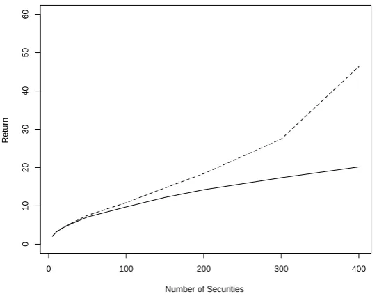
returns, ˆRp, for different values of p with the same sample size n = 500 in Figure 1. For
further evaluation, we depict the simulation theoretic optimal returns,R, and the plug-in
returns, ˆRp, in Table 1 for two different cases: (A) for different values ofp with the same
dimension-to-sample-size ratiop/n(= 0.5), and (B) for the same value of p(= 25215) but
different dimension-to-sample-size ratios p/n.
Place Figure 1 and Table 1 here
From Figure 1 and Table 1, we find the following: (1) both the plug-in return ˆRp
defined in (6) and its estimateRˆˆp defined in (7) are good estimates of the theoretic optimal
return R when p is small (≤ 30); (2) when p is large (≥ 60), the difference between the
theoretic optimal returnR and the plug-in return ˆRp (or Rˆˆp) becomes dramatically large;
(3) the larger the p, the greater the difference; and (4) when p is large, both the plug-in
return ˆRp and its estimate Rˆˆp are always larger than the theoretic optimal return, R,
computed by using the true mean and covariance matrix. These confirm the “Markowitz
optimization enigma” that the plug-in returns ˆRp should not be used in practice. In
addition, Figure 1 and Table 1 confirm a fairly high congruence between Rˆˆp and ˆRp for
all values of p. Hence, in this paper we will use ˆRp to represent both Rˆˆp and ˆRp if no
confusion occurs.
15
4.2
Bootstrap-Correction Method
In this section, our simulation is to show the superiority of both ˆRb and ˆcb over their
plug-in counterparts ˆRp and ˆcp. To this end, we first define the bootstrap-corrected
difference,dR
b, for the return as the difference between the bootstrap-corrected optimal
return estimate ˆRb and the theoretic optimal return R; that is,
dRb = ˆRb−R (13)
which will be used to compare the plug-in difference,
dRp = ˆRp−R (14)
for the return, where ˆRp and ˆRb are defined in (7) and (12), respectively.
To compare the bootstrapped allocation with the plug-in allocation, we define the
bootstrap-corrected difference norm,dc
b, and theplug-in difference norm, dcp, for
the allocations to be
dcb =∥ˆcb−c∥ and dcp =∥ˆcp−c∥, (15)
where dc
b is the difference norm between the bootstrap-corrected allocation ˆcb and the
theoretic optimal allocation c, while dc
p is the in difference norm between the
plug-in allocation ˆcp and the theoretic optimal allocation c. We then simulate 30 times to
compute dR
x and dcx for x = pand b, n = 500 and p= 100, 200 and 300. The results are
displayed in Table 2 and depicted in Figure 2.
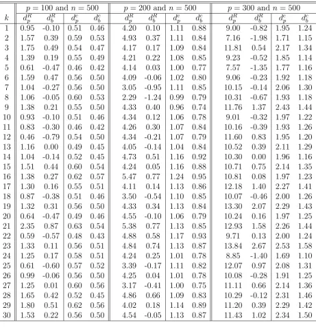
Place Figure 2 and Table 2 here
From Table 2 and Figure 2, we find the desired property that dR
b (dcb) is much smaller
than dR
p (dcp) in absolute value for all cases. This infers that the estimate obtained by
utilizing the bootstrap-corrected method is much more accurate in estimating the theoretic
two lines ofdR
p and dRb (or dcp anddcb) on each level as shown in Figure 2 separate further,
implying that the magnitude of improvement from dR
p (dcp) to dRb (dcb) is remarkable.
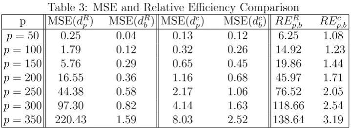
To further illustrate the superiority of our estimate over the traditional plug-in
es-timate, we present in Table 3 the mean square errors (MSEs) of the different estimates
for different p and plot these values in Figure 3. In addition, we define their relative
efficiencies (REs) for both allocations and returns to be
REp,bc = M SE(d
c p)
M SE(dc
b)
and REp,bR = M SE(d
R p)
M SE(dR
b)
. (16)
and report their values in Table 3.
Comparing the MSE ofdR
b (dcb) with that ofdRp (dcp) in Table 3 and Figure 3, the MSEs
of both dR
b and dcb have been reduced dramatically from those of dRp and dcp, indicating
that our proposed estimates are superior. We find that the MSE of dR
b is only 0.04,
improving 6.25 times from that ofdR
p whenp= 50. When the number of assets increases,
the improvement becomes much more substantial. For example, when p= 350, the MSE
of dR
b is only 1.59 but the MSE of dRp is 220.43, improving 138.64 times from that of dRp.
This is an unbelievable improvement. We note that when both n and p are bigger, the
relative efficiency of our proposed estimate over the traditional plug-in estimate could be
much larger. On the other hand, the improvement from dc
p todcb is also tremendous.
Place Table 3 and Figure 3 here
5
ILLUSTRATION
We illustrate the superiority of our approach by comparing the estimates of the
bootstrap-corrected return and the plug-in return for daily S&P500 data. To match our simulation
of n = 500 as shown in Table 1 and Figure 1, we choose 500 daily data backward from
December 30, 2005, for all companies listed in the S&P500 as the database for our
select p stocks from the S&P500 database randomly without replacement and compute
the plug-in return and the corresponding bootstrap-corrected return. We plot the plug-in
returns and the corresponding bootstrap-corrected returns in Figure 4 and report these
returns and their ratios in Table 4 for differentp. We also repeat the procedure (m=) 10
and 100 times for checking. For each m and for each p, we first compute the
bootstrap-corrected returns and the plug-in returns. Thereafter, we compute their averages for both
the bootstrap-corrected returns and the plug-in returns and plot these values in Panels 2
and 3 of Figure 4, respectively for comparison with the results in Panel 1 form = 1.
Place Table 4 and Figure 4 here
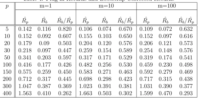
From Table 4 and Figure 4, we find that as the number of assets increases, (1) the
values of the estimates from both the bootstrap-corrected returns and the plug-in returns
for the S&P500 database increase, and (2) the values of the estimates of the plug-in
returns increase much faster than those of the bootstrap-corrected returns and thus their
differences become wider. These empirical findings are consistent with the theoretical
discovery of the “Markowitz optimization enigma” that the estimated plug-in return is
always larger than its theoretical value and their difference becomes larger when the
number of assets is large.
Comparing Figures 4 and 1 (or Tables 4 and 1), one will find that the shapes of the
graphs of both the bootstrap-corrected returns and the corresponding plug-in returns are
similar to those in Figure 1. This infers that our empirical findings based on the S&P500
are consistent with our theoretical and simulation results, which, in turn, confirms that
our proposed bootstrap-corrected return performs better.
One may doubt the existence of bias in our sampling as we choose only one sample
in the analysis. To circumvent this problem, we, in addition, repeat the procedure m
(=10, 100) times. For eachmand for eachp, we compute the bootstrap-corrected returns
returns and the plug-in returns. Thereafter, we plot the averages of the returns in Figure
4 and report these averages and their ratios in Table 4 for m = 10 and 100. When
comparing the values of the returns for m = 10 and 100 with m = 1, we find that the
plots are basically of the similar values for eachpbut become smoother, inferring that the
sampling bias has been eliminated by increasing the number ofm. The results form= 10
and 100 are also consistent with the plot in Figure 1 in our simulation, inferring that our
bootstrap-corrected return is a better estimate for the theoretical return in the sense that
its value is much closer to the theoretical return when compared with the corresponding
plug-in return.
6
CONCLUSION
Being of both theoretical and practical interest, the basic problem for MV analysis is
identifying those combinations of assets that constitute attainable efficient portfolios.
Unfortunately, there are problems that accompany any MV analysis. With this in mind,
this paper sets out to solve this dilemma by developing a new optimal return estimate
to capture the essence of portfolio selection. Since our approach is easy to operate and
implement in practice, the whole efficient frontier of our estimates can be constructed
analytically. Thus, our proposed estimator facilitates the Markowitz MV optimization
procedure, making it implementable and practically useful.
Since our model includes the situation in which one of the assets is a riskless asset,
the separation theorem holds and thus our proposed return estimate is the optimal
com-bination of the riskless asset and the optimal risky portfolio. We further note that the
other assets listed in our model could be common stocks, preferred shares, bonds, and
other types of assets so that the optimal return estimate proposed in our paper actually
represents the optimal return for the best combination of riskless rate, bonds, stocks, and
For instance, the optimization problem can be formulated with short-sales restrictions,
trading costs, liquidity constraints, turnover constraints, and budget constraints;16 see,
for example, Detemple and Rindisbacher (2005), Muthuraman and Kumar (2006), and
Lakner and Nygren (2006). Each of these constraints leads back to a different model for
determining the shape, composition, and characteristics of the efficient frontier and,
there-after, makes MV optimization a more flexible tool. For example, Xia (2005) investigates
the problem with a non-negative wealth constraint in a semimartingale model. Another
direction for further research is to adopt the continuous-time multiperiod Markowitz’s
problem (see, for example, Li and Ng (2000), Emmer, Kl¨uppelberg, and Korn (2001)
and Xia and Yan (2006) for details on the issue). Further research could also include
conducting an extensive analysis to compare the performance of our estimators with
other state-of-the-art estimators in the literature, for example, factor models or Bayesian
shrinkage estimators.
We note that the returns being studied in the MV optimization procedure are usually
assumed to be normally distributed. However, many studies (for example, see Fama
(1963, 1965), Blattberg and Gonedes (1974), Clark (1973), and Fielitz and Rozelle (1983))
conclude that the normality assumption in the distribution of a security or portfolio return
is violated. We further note that another contribution of our proposed approach is that
we relax the normality assumption in the underlying distribution for the return being
studied in the MV optimization procedure. In addition, we relax the condition to the
existence of the second moments for some cases and to the fourth moments for some
other cases. The returns could follow any distribution, and furthermore, they are not
necessarily identically-distributed in our proposed approach.
We note that Leung, et al. (2012) provide a close form estimation for Bai et al. (2009a)
while Bai, et al. (2013, 2016) further extend the work by developing the theory of
spectral-corrected estimation. They first establish a theorem to explain why the plug-in return
16
greatly overestimates the theoretical optimal return. Thereafter, they prove that under
some situations the plug-in return is√γ times bigger than the theoretical optimal return,
while under other situations, the plug-in return is bigger than but may not be√γ times
larger than its theoretic counterpart where γ = 1
1−y with y being the limit of the ratio
p/n. They then develop the spectral-corrected estimation for the Markowitz MV model
which performs much better than both the plug-in estimation and the bootstrap-corrected
estimation not only in terms of the return but also in terms of the allocation and the risk.
They also develop properties for their proposed estimation and conduct a simulation to
examine the performance of their proposed estimation. Their simulation shows that their
proposed estimation not only overcomes the problem of “over-prediction,” but also
cir-cumvents the “under-prediction,” “allocation estimation,” and “risk” problems. Their
simulation also shows that their proposed spectral-corrected estimation is stable for
dif-ferent values of sample size n, dimension p, and their ratio p/n. In addition, they relax
the normality assumption in our proposed estimation so that their proposed
spectral-corrected estimators could be obtained when the returns of the assets being studied could
follow any distribution under the condition of the existence of the fourth moments.
Finally, we note that the approach developed in this paper is useful in empirical
stud-ies, for example, Abid, et al. (2014) apply the approach developed in the paper to examine
preferences for international diversification versus domestic diversification from American
investors’ viewpoints. On the other hand, Hoang, et al. (2015) apply the approach
devel-oped in the paper to study the role of gold quoted on the Shanghai Gold Exchange in the
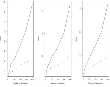
Figure 1: Empirical and theoretical optimal returns for different numbers of assets
0 100 200 300 400
0
10
20
30
40
50
60
Number of Securities
Return
Solid line — the theoretic optimal return (R); Dashed line—the plug-in return ( ˆRp);
Dotted line— the estimate of plug-in return (Rˆˆp).
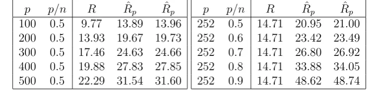
Table 1: Performance of ˆRp and Rˆˆp over the Optimal Return R for different values of p
and for different values of p/n
p p/n R Rˆp Rˆˆp
100 0.5 9.77 13.89 13.96 200 0.5 13.93 19.67 19.73 300 0.5 17.46 24.63 24.66 400 0.5 19.88 27.83 27.85 500 0.5 22.29 31.54 31.60
p p/n R Rˆp Rˆˆp
252 0.5 14.71 20.95 21.00 252 0.6 14.71 23.42 23.49 252 0.7 14.71 26.80 26.92 252 0.8 14.71 33.88 34.05 252 0.9 14.71 48.62 48.74
Note: The table compares the performance between ˆRp andRˆˆp for samep/n ratio with
different numbers of assets,p, and for same pwith different p/n ratio wheren is number of sample,R is the optimal return defined in (1), ˆRp and Rˆˆp are defined in (6) and (7),
Figure 2: Comparison between the Empirical and Corrected Portfolio Allocations and Returns
Number of Simulation
Difference Comparison
0 5 10 15 20 25 30
0
5
10
15
p=300,return comparison
0 5 10 15 20 25 30
0.0 0.5 1.0 1.5 2.0 2.5 p=300,allocation comparison
0 5 10 15 20 25 30
0
5
10
15
p=200,return comparison
0 5 10 15 20 25 30
0.0 0.5 1.0 1.5 2.0 2.5 p=200,allocation comparison
0 5 10 15 20 25 30
0
5
10
15
p=100,return comparison
0 5 10 15 20 25 30
0.0 0.5 1.0 1.5 2.0 2.5 p=100,allocation comparison
Solid line —the absolute value ofdc
p anddRp respectively;
Dashed line— the absolute value ofdc b andd
R
b respectively.
Table 2: Comparison between the Empirical and Corrected Portfolio Returns and Allo-cations
p= 100 and n= 500 p= 200 and n = 500 p= 300 and n= 500
k dR
p dRb dcp dcb dRp dRb dcp dcb dRp dRb dcp dcb
1 0.95 -0.10 0.51 0.46 4.20 0.10 1.11 0.88 9.00 -0.82 1.95 1.24 2 1.57 0.39 0.59 0.53 4.93 0.37 1.11 0.84 7.16 -1.98 1.71 1.15 3 1.75 0.49 0.54 0.47 4.17 0.17 1.09 0.84 11.81 0.54 2.17 1.34 4 1.39 0.19 0.55 0.49 4.21 0.22 1.08 0.85 9.23 -0.52 1.85 1.14 5 0.61 -0.47 0.46 0.42 4.14 0.03 1.00 0.77 7.57 -1.35 1.77 1.16 6 1.59 0.47 0.56 0.50 4.09 -0.06 1.02 0.80 9.06 -0.23 1.92 1.18 7 1.04 -0.27 0.56 0.50 3.05 -0.95 1.11 0.85 10.15 -0.14 2.06 1.30 8 1.06 -0.05 0.60 0.53 2.29 -1.24 0.99 0.79 10.31 -0.67 1.93 1.18 9 1.38 0.21 0.55 0.50 4.33 0.40 0.96 0.74 11.76 1.37 2.43 1.44 10 0.93 -0.10 0.51 0.46 4.34 0.12 1.06 0.78 9.01 -0.32 1.97 1.22 11 0.83 -0.30 0.46 0.42 4.26 0.30 1.07 0.84 10.16 -0.39 1.93 1.26 12 0.46 -0.79 0.54 0.50 4.34 -0.21 1.07 0.79 11.60 0.83 1.95 1.20 13 1.16 0.00 0.49 0.45 4.05 -0.14 1.04 0.84 10.52 0.39 2.11 1.29 14 1.04 -0.14 0.52 0.45 4.73 0.51 1.16 0.92 10.30 0.00 1.96 1.16 15 1.51 0.44 0.60 0.54 4.24 0.05 1.16 0.88 10.71 0.75 2.14 1.35 16 1.38 0.27 0.62 0.57 5.47 0.77 1.24 0.95 10.81 0.08 1.97 1.23 17 1.30 0.16 0.55 0.51 4.11 0.14 1.13 0.86 12.18 1.40 2.27 1.41 18 0.87 -0.38 0.51 0.46 3.50 -0.54 1.10 0.85 10.07 -0.46 2.00 1.26 19 1.32 0.31 0.56 0.50 4.33 0.34 1.13 0.84 13.30 2.07 2.29 1.43 20 0.64 -0.47 0.49 0.46 4.55 -0.10 1.06 0.79 10.24 0.16 1.97 1.25 21 2.35 0.87 0.63 0.54 5.38 0.77 1.13 0.85 12.93 1.58 2.26 1.44 22 0.59 -0.57 0.48 0.43 4.88 0.58 1.17 0.93 9.71 0.13 2.00 1.24 23 1.33 0.11 0.56 0.51 4.84 0.74 1.13 0.87 13.84 2.67 2.53 1.58 24 1.25 0.17 0.58 0.51 4.24 0.25 1.01 0.78 8.85 -1.40 1.69 1.10 25 0.61 -0.60 0.57 0.52 3.39 -0.17 1.11 0.82 12.07 0.97 2.08 1.31 26 0.99 -0.06 0.56 0.50 4.25 0.04 1.01 0.78 10.08 -0.28 1.91 1.25 27 1.25 0.01 0.60 0.56 3.17 -0.41 1.00 0.75 11.11 0.66 2.14 1.36 28 1.65 0.42 0.52 0.45 4.86 0.66 1.09 0.83 10.29 -0.12 2.31 1.46 29 1.80 0.51 0.62 0.56 4.02 0.18 1.14 0.89 11.20 0.39 2.29 1.42 30 1.53 0.22 0.56 0.50 4.54 -0.05 1.13 0.87 11.43 1.02 2.34 1.50
Table 3: MSE and Relative Efficiency Comparison p MSE(dR
p) MSE(dRb ) MSE(dcp) MSE(dcb) REp,bR REp,bc
p= 50 0.25 0.04 0.13 0.12 6.25 1.08
p= 100 1.79 0.12 0.32 0.26 14.92 1.23
p= 150 5.76 0.29 0.65 0.45 19.86 1.44
p= 200 16.55 0.36 1.16 0.68 45.97 1.71
p= 250 44.38 0.58 2.17 1.06 76.52 2.05
p= 300 97.30 0.82 4.14 1.63 118.66 2.54
p= 350 220.43 1.59 8.03 2.52 138.64 3.19
Figure 3: MSE Comparison between the Empirical and Corrected Portfolio Alloca-tions/Returns
50 100 200 300
0
50
100
150
200
Number of Securities
MSE for Return Difference
50 100 200 300
0
2
4
6
8
Number of Securities
MSE for Allocation Difference
Solid Line — the MSE ofdR p andd
c
p, respectively;
Dashed line — the MSE ofdR b andd
c
b, respectively.
Note: The plots on the left are the plots of the MSEs for dR
p and dRb , while the plots on the
right are the plots of the MSEs fordc
p and dcb, respectively. dRb,dRp,dcb and dcp are defined in
[image:37.595.119.466.244.522.2]Figure 4: Comparison between the Plug-in Returns and Bootstrap-Corrected Returns
0 100 200 300 400
0.2
0.4
0.6
0.8
1.0
1.2
1.4
1.6
Number of Securities
Return
0 100 200 300 400
0.5
1.0
1.5
Number of Securities
Return
0 100 200 300 400
0.5
1.0
1.5
Number of Securities
Return
Solid line —Plug-in Return;
Dashed line— Bootstrap-Corrected Return.
Table 4: Plug-in Returns and Bootstrap-Corrected Returns
p m=1 m=10 m=100
ˆ
Rp Rˆb Rˆb/Rˆp Rˆp Rˆb Rˆb/Rˆp Rˆp Rˆb Rˆb/Rˆp
5 0.142 0.116 0.820 0.106 0.074 0.670 0.109 0.072 0.632 10 0.152 0.092 0.607 0.155 0.103 0.650 0.152 0.097 0.616 20 0.179 0.09 0.503 0.204 0.120 0.576 0.206 0.121 0.573 30 0.218 0.097 0.447 0.259 0.154 0.589 0.254 0.148 0.576 50 0.341 0.203 0.597 0.317 0.171 0.529 0.319 0.174 0.541 100 0.416 0.177 0.426 0.482 0.256 0.530 0.459 0.230 0.498 150 0.575 0.259 0.450 0.583 0.271 0.463 0.592 0.279 0.469 200 0.712 0.317 0.445 0.698 0.298 0.423 0.717 0.315 0.438 300 1.047 0.387 0.369 1.023 0.391 0.381 1.031 0.390 0.377 400 1.563 0.410 0.262 1.663 0.503 0.302 1.599 0.470 0.293
Note: ˆRp and ˆRb are defined in (7) and (12), respectively.
REFERENCES
ABID, F., P.L. LEUNG, M. MROUA, and W.K. WONG, (2014):
Interna-tional Diversification versus Domestic diversification: Mean-Variance
Port-folio Optimization and stochastic dominance approaches, Journal of Risk
and Financial Management, 7(2), 45-66.
A¨IT SAHALIA, Y., and M. BRANDT, (2001): Variable Selection for Portfolio
Choice, Journal of Finance56, 1297-1351.
BAI, Z.D., (1999): Methodologies in Spectral Analysis of Large Dimensional
Random Matrices, A Review, Statistica Sinica 9, 611-677.
BAI, Z.D., H. LI, M.J. MCALEER, and W.K. WONG, (2016):
Spectrally-Corrected Estimation for High-Dimensional Markowitz Mean-Variance
Op-timization, Econometric Institute Research Papers EI2016-20, Erasmus
University Rotterdam, Erasmus School of Economics (ESE),