An approximate dynamic programming approach
to the micro-CHP scheduling problem
Maarten Vinke
August 24, 2012
Abstract
Due to environmental issues such as the greenhouse effect, and the fact that the earth’s oil and gas reserves are slowly depleting, the electricity supply chain is slowly trans-forming toward novel methods of energy generation. One of these methods consists of using CHPs in households to satisfy part of the electricity demand. A micro-CHP is an installation that simultaneously generates heat and electricity, replacing the traditional boiler. In this setting, the electricity production is essentially a by-product of the heat production, so that there is no heat loss during the electricity production process. The micro-CHP comes with a heat buffer, in which hot water can be stored, so there is some flexibility in the time for this production.
Still, as electricity is dependent on the heat demand, the electricity generation from a single house can become erratic. Therefore, in this thesis we consider a group of houses, for which the goal is to obtain a more or less constant electricity production. To enforce this, we assume that there are fixed upper and lower bounds on the to-tal electricity production. The goal in this thesis is to find a production schedule for the different micro-CHPs, so that both these total electricity bounds and the houses’ individual heat demands are satisfied. Within these constraints, the objective is to max-imize the revenue gained by selling this electricity, whereby these electricity prices are time-dependent, with peaks during the hours when electricity demand is higher.
This micro-CHP problem has already been investigated by Bosman [4], where mul-tiple heuristics were used to find such a schedule, using a discretized time scale. In this thesis, we have attempted to solve the scheduling problem mentioned above using the technique of Approximate Dynamic Programming (ADP). For this the problem was first modelled as a Dynamic Program, which was too large to solve exactly.
After this technique is introduced by considering the taxicab problem, it is used on the actual micro-CHP problem. As a decision here consists of determining which micro-CHPs are turned on and off in the following time interval, often the number of possible decisions is too large to consider them all. Therefore, first the decision space is reduced by using a strict priority list. Then an approximation function for every state is defined, which uses a weighted sum of basis functions. These basis functions are numerical values based on certain features of a state. Then, the approximation function and the reduced decision space can be used to find to find paths through the state space, each resulting in a production schedule for the micro-CHPs. After such a schedule has been found, the values found in this schedule are used to update the weights in the approximation function, to increase the quality of the approximation. This is repeated for multiple iterations.
Dankwoord
Dit afstudeerwerk had ik uiteraard nooit alleen kunnen volbrengen. Daarom wil ik allereerst mijn beide begeleiders bedanken. Maurice Bosman heeft mij vooral geholpen met het invoeren van de data, het inwerken in het onderwerp en met mijn verslag. Uiteraard heb ik ook heel veel gehad aan de informatie en data uit zijn afstudeerscriptie, en de daaraan voorafgaande papers. Johann Hurink wil ik vooral bedanken voor de hulp met het schrijven van mijn verslag. Regelmatig heeft hij mijn verslag doorgeploegd, en meer dan eens stonden daarna op sommige pagina’s meer aantekeningen dan originele tekst. Dit zag er altijd wat deprimerend uit, maar uiteindelijk is het mijn verslag wel enorm ten goede gekomen. Daarnaast wil ik ook Jan-Kees van Ommeren bedanken voor het plaatsnemen in mijn afstudeercommissie.
Contents
1 Introduction 5
2 The Micro-CHP problem 7
2.1 Modelling the micro-CHP . . . 7
2.1.1 Decision variables and streak values . . . 8
2.1.2 The heat behaviour . . . 9
2.1.3 Electricity bounds . . . 10
2.1.4 Objective . . . 10
2.1.5 The full model . . . 10
2.2 DP model for a single house . . . 11
2.2.1 Re-expressing the heat level . . . 11
2.2.2 States, decisions and transitions . . . 16
2.2.3 The value function . . . 17
2.3 The problem for multiple houses . . . 18
2.3.1 New states, decisions and transitions . . . 18
2.3.2 The new value function . . . 18
3 The taxicab problem 19 3.1 Introduction to Dynamic Programming . . . 19
3.2 The taxicab problem . . . 21
3.3 ADP for the taxicab problem . . . 22
3.3.1 Updating the value function . . . 23
3.3.2 Finding the path . . . 23
3.4 Results and analysis . . . 25
3.4.1 Grid 1 . . . 28
3.4.2 Grid 2 . . . 28
3.4.3 Grid 3 . . . 31
3.5 Conclusion . . . 33
4 ADP Approach 36 4.1 Reducing the decision space . . . 36
4.2 The value function . . . 37
4.2.1 Value function decomposition . . . 38
4.3 Finding a path . . . 40
5 Alternative approaches 43 5.1 ILP approach . . . 43
5.2 Solving the Dynamic Program . . . 43
5.3 DP-based Local Search . . . 43
6 Results 45
6.1 Small instances . . . 45
6.2 The choice ofα . . . 46
6.3 Large instances . . . 50
6.4 Basis functions . . . 55
6.5 Randomness . . . 56
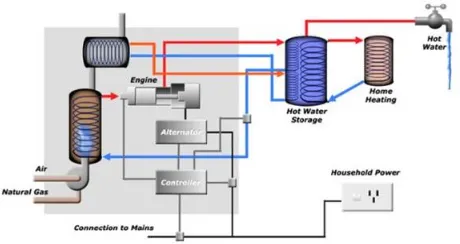
Figure 1: Example of a micro-CHP; the MTS Infinia micro-CHP
1
Introduction
Over the last years the demand for a more durable and efficient electricity generation is getting more and more attention. Partly because the demand for energy is increasing, and partly because the earth is running out of the traditional energy resources, such as oil and gas. In this thesis we look at one particular approach which can contribute to solving this problem, which is the micro-CHP. CHP here is an approximation for Combined Heat and Power. A micro-CHP is a special kind of boiler, that can be used within a household. As the abbreviation already suggests, the micro-CHP simultane-ously produced heat and power, or electricity. The heat can be used for hot water and central heating (if necessary), while the generated electricity used within the household or added to the network. A picture of a micro-CHP is shown in Figure 1.
With this micro-CHP it is possible to get a more efficient production of electricity than with a traditional power plant, because there the heat loss is greatly reduced, as the heat is used within the household. This leads to an energy efficiency of about 95 %, where e.g. an open-cycle gas turbine has only an efficiency of 35-42 % [5]. The functioning of a micro-CHP is shown schematically in Figure 2. Note that this combined generation implies that there is only electricity production when there is a demand for heat.
Still, there are some difficulties with this arrangement, because if electricity is only produced when there is a heat demand, the total electricity production from houses equipped with a micro-CHP becomes erratic and difficult to predict. To still have a possibility of steering the electricity production, every micro-CHP has a heat buffer where hot water can be stored, so that the production does have some flexibility in time.
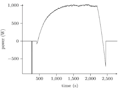
Figure 2: Schematic representation of a micro-CHP production process
if we consider a group of multiple houses equipped with a micro-CHP, we want to find a production schedule for the micro-CHPs. This schedule should ensure that the houses’ heat demands are fulfilled, and the electricity production performs along the lines of a desired, more or less constant, schedule.
This problem has already been investigated by Bosman [4], where several heuristics were used to solve this scheduling problem. In one of these approaches, this problem was modelled as a very large Dynamic Programming instance. In this thesis an attempt is made to solve this Dynamic Programming problem with Approximate Dynamic Pro-gramming (ADP).
The structure of this thesis is as follows:
In Section 2 the micro-CHP problem is explained, and it is described how this problem can be modelled as a (very large) dynamic programming problem, as was done in [4]. In Section 3 ADP is introduced using an easier problem; the taxicab problem. This problem can be solved using ADP, and has the advantage that the approach here is a lot more intuitive than for the micro-CHP problem. This is the reason that we take a small detour by examining the taxicab problem, to later draw similarities that can be used for the micro-CHP problem. In Section 4 we then return to the micro-CHP problem, and describe how ADP can be implemented in this problem.
2
The Micro-CHP problem
The micro-CHP is a boiler that produces both heat and electricity, that can be used within a house. In this thesis, we consider a situation with a group of houses that are all equipped with a micro-CHP. For every house, the heat necessary for heating the house and hot water has to come from the micro-CHP. We assume that the heat profile is known for every house, meaning that for different time intervals it is specified how much heat is required. Furthermore, every house has a heat buffer, in which it can store up to a certain amount of heat, in the form of hot water.
Of course, we will not know exactly how much heat the houses need, and when they need it. In this thesis, we assume that an estimation is known for this, based on previous heat data for the house. The deviations from this estimation are resolved by using a real-time control, for which also some additional space in the heat buffer is reserved. The real-time control will follow the original schedule as close as possible. This means that for our scheduling problem, we can assume the estimations of the heat demand to be fixed demands.
For this group of houses, it is assumed that a power company has set upper and lower bounds for the total production of electricity for different intervals. This is done to force the group to behave in a more predictable manner, which makes it easier for the company to deal with the total electricity produced by the group. A group of houses which behaves in such a way is called a virtual power plant (VPP).
The power company pays the group for the electricity produced, where the price of electricity is time-dependent.
The goal is now to maximize the revenue of the electricity sales of the group of houses, while respecting the upper and lower bound given by the power company, and while satisfying the heat demands of the different houses.
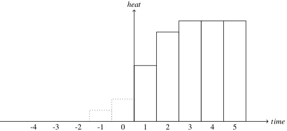
In doing this, the behaviour of the micro-CHP also has to be considered. First, there is only one level of production, so the micro-CHP either runs at full force or it is turned off; it can not run at half force. A typical electricity production scheme of a micro-CHP is shown in Figure 3. Here we can see that the electricity generation of the micro-CHP slowly builds up to a near-constant maximum production level, and that also some energy is generated during shutdown. After shutdown, the micro-CHP needs to cool down. Because of this, and to ensure that the micro-CHP runs are efficient, we infer that the micro-CHP has fixed start-up and shutdown periods. These cannot be interrupted, and are typically longer than the time needed to reach the maximum production or to stop producing.
In the next subsection this micro-CHP problem is translated into a mathematical model. After that, this model is transformed into a Dynamic Programming problem. This is first done for a single house, after which this is extended to multiple houses.
2.1
Modelling the micro-CHP
Figure 3: Generation during a micro-CHP run
within a time interval is constant. We hereby consider a micro-CHP to be turned off while it is shutting down, and during the start-up it is considered on.
2.1.1 Decision variables and streak values
To keep track of the status of the micro-CHPs, we introduce binary decision variables xi,t. These are defined as follows:
xi,t=
0 if the micro-CHP in houseiis turned off during intervalt
1 if the micro-CHP in houseiis turned on during intervalt. (1)
As can be seen from Figure 3, the production level of a micro-CHP depends on how long the micro-CHP has been running, or how long it has been off (if it is still in the process of shutting down). This indicates that it is useful to keep track of this running time. For this we introduce variablesai,twith the following definition:
ai,t=
# of intervals the micro-CHP has been turned on consecutively ifxi,t=1 - # of intervals the micro-CHP has been off consecutively ifxi,t=0.
(2) We refer toai,t as the ”streak value” of houseiin intervalt. This streak value is taken at the end of the intervalt. In this way by choosingt=0, we can specify also the situation at the beginning of the planning horizon, meaning thatai,0∈Z\{0}is a
model parameter that describes the initial streak value of the micro-CHP in housei. The streak values and the decision variablesxi,t are linked by the following relation:
ai,t=
max(ai,t−1+1,1) ifxi,t=1
This holds as the number of consecutive intervals is increased by 1 if the on/off status is the same as in the previous interval. When it is different, a new streak is started, starting from 1 or−1.
From (3) it follows that the ai,t are completely determined by the xi,t variables, for allt>0, asai,0is a fixed parameter. With these streak values we can also make
sure that the start-up and shutdown periods are respected. Let the number of intervals during which the micro-CHP be denoted byTon, and the number of intervals required for shutdown byToff. With these notations we impose the following constraints on the model:
xi,t=1 if 1≤ai,t−1<Ton ∀i∈ {1,2, ..,N},t∈ {1,2, ...,T}
xi,t=0 if −1≥ai,t−1>−Toff ∀i∈ {1,2, ..,N},t∈ {1,2, ...,T}. (4)
2.1.2 The heat behaviour
We consider the heat behaviour in a single house. As mentioned in the introduction, the heat in each house is produced by the micro-CHP, and can be stored in a buffer. For this buffer there are upper and lower bounds for the amount of heat that can be stored. We assume that the lower bound is 0, and denote the upper bound of the heat buffer in houseibyLmax,i. To keep track of the amount of heat in the buffer of houseiat the end of intervalt, we introduce the variableLi,t,t∈ {0,1,2, ...,T}. This variable is defined as the amount of heat in houseiat the end of intervalt, and is referred to as the ”heat level” of houseiin intervalt. We assume that the heat level at the beginning of the planning interval,L0,tis known. During intervaltwithin the planning horizon, the heat level in houseiis changed by the following factors:
• The house may use some up some heat for heating or hot water. As explained be-fore, we assume that the heat demands are fixed, and useDitfor the given amount of heat that house i needs during intervalt. The valuesDit, i∈ {1,2, ...,N}, t∈ {1,2, ...,T}are known model parameters.
• The micro-CHP can produce some heat during intervalt, which is put into the buffer. As the production rate cannot be controlled, the heat production only depends on how long the micro-CHP has been on in intervalt, and thus on the streak valueai,t of the micro-CHP. Therefore we can write the heat production in houseiduring intervalt asP(ai,t), representing the production of heat corre-sponding to a streak value ofai,t.
Now, if the streak valueai,t and the heat level at the previous interval Li,t−1 are
known, the heat level after intervalt Li,tcan be found using the following relation:
Li,t=Li,t−1+P(ai,t)−HLi−Dit ∀i∈ {1,2, ..,N},t∈ {1,2, ...,T} (5) In this formulaHLiandDit are fixed model parameters, whileP(ai,t)depends on the decision variables. To make sure that heat level does not exceed the maximum amount of heat that can be stored, and that there is always enough heat to meet the demands, the following constraints are imposed:
0≤Li,t≤Lmax,i ∀i∈ {1,2, ...,N},t∈ {1,2, ...,T}. (6) 2.1.3 Electricity bounds
The electricity production has to be taken into account as well. Similar to the heat production, the electricity generationEi,tin houseiduring intervaltalso only depends on the streak valueai,t, and can be written as Ei,t =E(ai,t). As mentioned in the introduction, there are fixed upper and lower bounds for the total electricity generation of the fleet in each intervalt, which are denoted byEmin,t andEmax,t. This leads to the following constraints for the total electricity generation:
Emin,t≤ N
∑
i=1
E(ai,t)≤Emax,t ∀t∈ {1,2, ...,T}. (7)
2.1.4 Objective
The constraints (3) to (7) restrict the possible choices for the decision variables. Within these constraints, the objective is to maximize the total revenue over all intervals gained from selling the electricity. If we denote the price of electricity during intervalt by Pr(t), this revenue can be written as
T
∑
t=1 (Pr(t)
N
∑
i=1
E(ai,t)) (8)
2.1.5 The full model
max T
∑
t=1 (Pr(t)
N
∑
i=1
E(ai,t))
under the constraints:
xi,t∈ {0,1} ∀i,t ai,t=
max(ai,t−1+1,1)ifxi,t=1 min(−1,ai,t−1−1)ifxi,t=0
∀i,t xi,t=1 if 1≤ai,t−1<Ton ∀i,t xi,t=0 if −Toff <ai,t−1≤ −1 ∀i,t
Li,t=Li,t−1+P(ai,t)−HLi,t−Di,t ∀i,t 0≤Li,t≤Lmax,i ∀i,t Emin,t≤
N
∑
i=1
E(ai,t)≤Emax,t ∀t (9)
Written this way, this problem comes down to a constrained optimisation problem. In Bosman [4] this problem was proven to be NP-hard over the number of housesN by reduction to 3-partition, which means there is in general no fast solution for larger instances this problem.
With some clever reformulations, this problem can also be written as an Integer Linear Programming problem, as has been done by Bosman et al. in [1]. However, in this thesis this problem is transformed to a Dynamic Programming instance, so that ADP can be applied to this problem.
2.2
DP model for a single house
To get an idea of how the micro-CHP problem can be solved using Dynamic Program-ming, we first consider this problem with only one house. The single house problem is a lot easier to grasp, and can easily be expanded to the problem for multiple houses. For convenience, we remove theifrom the subscript of the variables and parameters. Also, for now we disregard the global electricity constraint (7).
In applying Dynamic Programming to this model, we use the intervalst for the phases of the problem. In every phaset,t∈0,1, ...,T−1 the value ofxt+1is chosen.
From the constraints it follows thatat andLt follow directly from the sequence ofxt, and so the choice of thext defines the entire solution.
2.2.1 Re-expressing the heat level
time heat
P(1) P(2) P(−1)
1 2 3 4 5 6 7 8 9 10 11
Hmax
Ton kr Toff
[image:13.612.140.451.127.300.2]Hon kr·Hmax Hoff
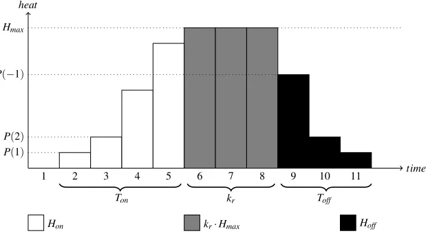
Figure 4: Example of a micro-CHP run
Yet, asLtis a continuous variable, we can not just write down all possible combi-nations ofatandLtto describe the states, as we need them for Dynamic Programming. Therefore we introduce two discrete variables to characterize the heat level at timet: bt, the total number of time intervals the micro-CHP has been turned on up to timet, andct, the number of times the micro-CHP was switched off. Hereby an off-switch means that the micro-CHP was turned fromontooff.
To clarify howLtcan be found from these values, we look at the heat generated in a typical runr, as shown in Figure 4. First, in every run, the micro-CHP has a start-up period ofTonintervals. Similarly,Toff intervals are used to shut down the micro-CHP. We defineHon:=∑Ti=on1P(i)as the total heat produced during a complete start-up, and
Hoff :=∑−i=1−ToffP(i)as the heat produced while shutting down. In between these
start-up and shutdown periods, the maximum heat productionHmaxis produced in each time interval. If we denote bykrthe number of intervals in runrat which the micro-CHP remains switched on after the minimum on time, the total production during runrof a micro-CHP can be written asHon+kr·Hmax+Hoff.
As introduced above, we denote byct the total number of off-switches up to time t, which also represents the number of runs that have finished within the planning interval. For now we assume that each of these off-switches corresponds to a completed run which is entirely inside the planning interval. To find the amount ofon-intervals during these runs, we define a parameter ˜btdescribing the total on time during the first ctruns, which are already completed. ˜bt can be found as follows:
˜ bt=
bt−at ifat>0 bt ifat<0
(10)
-4 -3 -2 -1 0 1 2 3 4 5 time
[image:14.612.133.424.127.260.2]heat
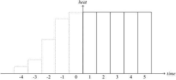
Figure 5: Example of the beginning phase of the planning horizon;a0≥Ton
the firstctcompleted runs,Hc, equals:
Hc = ∑cr=t 1(Hon+Hoff+kr·Hmax) =ct·(Hon+Hoff) +Hmax∑cr=t 1kr =ct·(Hon+Hoff) +Hmax·(bt˜ −ctTon)
(11)
We get the last equation from observing that the ˜bt on-intervals are used for either start-up intervals or maximum production intervals. As the total number of intervals used for start-up equalsctTon, the number of maximum production intervals∑cr=t 1kr equals ˜bt−ctTon.
However, we still need to deal with the assumptions we have made. First of all, we consider the assumption that each of thect runs was entirely in the planning horizon. This is not always true for the first run, which may have started before time 0, nor for the last run, that may still be in the process of shutting down. Also, a new run could have started after runct. Because of this, we use correction factorsHstart to correct Hc for the first run, andHend to correct for the last run. Hereby we assume that the micro-CHP was turned off during at least one interval after interval 0, which can also be written asat<t. Forat≥t, we perform a separate calculation. In findingHstartwe consider four different cases, based on the value of the streak value at the beginning of the planning horizona0:
• Ifa0≥Ton, the micro-CHP was turned on initially, and the start-up of the first run was already completed during interval 1. Therefore the start-up intervals of the first run should not be considered in finding the total heat production. Instead, these intervals have to be counted as maximum production intervals. As the entire start-up happened before the first interval, the intervals of one start-up have to be replaced by maximum production intervals, as in Figure 5. In this case the correction factor equalsTonHmax−Hon.
• If 0<a0<Ton, as depicted in Figure 6, only the firsta0start-up intervals were
-4 -3 -2 -1 0 1 2 3 4 5 time
[image:15.612.134.425.126.259.2]heat
Figure 6: Example of the beginning phase of the planning horizon; 0<a0<Ton
-4 -3 -2 -1 0 1 2 3 4 5 time
heat
Figure 7: Example of the beginning phase of the planning horizon;−Tmathito f f<a0<0
production intervals. As the heat produced before interval 1 equals∑ai=01P(i), the
correction factor is equal toa0Hmax−∑ai=01P(i).
• If−Toff <a0,t<0, the micro-CHP was switched off in interval 0, but was still producing some heat as it is shutting down (see Figure 7). Since the off-switch of that run occurred before interval 1 it is not included inct. Therefore, in this case an extra amount of heat of∑ai=0−−1ToffP(i)needs to be added.
• Finally, ifa0<−Toff, we have a situation similar to Figure 4, and no alterations onHcare necessary.
Combining these observations, we get:
Hstart=
TonHmax−Hon ifa0>Ton
a0Hmax−∑ai=01P(i) if 1≤a0≤Ton
∑ai=0−−1ToffP(i) if −Toff ≤a0≤0
0 ifa0<−Toff
[image:15.612.139.402.297.432.2]...
t-3 t-2 t-1 t t+1 t+2 time
[image:16.612.141.340.183.317.2]heat
Figure 8: Example of the final phase of the planning horizon;at>0
...
t-3 t-2 t-1 t t+1 t+2 time
heat
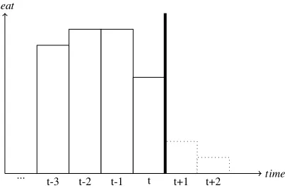
[image:16.612.140.343.459.592.2]To calculateHend(at)we consider different three different scenarios for the values ofat:
• The situation whereat>0 is depicted in Figure 8. As the production intervals of the current run were not considered inHcby the definition of ˜bt in (10), the correction consists of the heat produced during the last run:∑ai=t1P(i). Note that this heat was all produced after interval 1, as we assumed that the micro-CHP has been off at some interval up to timet.
• IfToff <at<0, the shutdown of the last run was not completed, as can be seen in Figure 9. To correct for that, an amount of∑ai=t−−1ToffP(i)heat has to be subtracted
fromHc.
• Ifat<−Toff, the last run has been completed, and no correction is necessary. This results in the following expression forHend:
Hend=
∑ai=t1P(i) ifat>0
−∑ai=t−−1ToffP(i) if −Toff <at<0
0 ifat<−Toff
(13)
With these correction factors, the total heat produced up to timet,Htotal, can be found. For this, ifat<t, we can use the sum ofHc(t)and the correction factors we have just defined. Ifat≥tthe micro-CHP has been on at all intervals, so the heat produced is just the part of the current run starting from interval 1, which equals∑ai=at 0+1P(i).
Using this, we can now expressHtotalas follows:
Htotal=
∑ai=at 0+1P(i) ifat≥t
Hc(t) +Hstart+Hend ifat<t
(14)
As all values used in the expression above can be derived fromat,btandct,Htotalis also a function of these three variables. As the heat lossesHLi,tand the heat demands Di,t are model parameters, we can find the heat level at timet fromat,bt andct as follows:
Lt:=L0+Htotal− t
∑
i=1
(HLi,t+Di,t) (15)
2.2.2 States, decisions and transitions
AsLt can be found from at,bt andct, and asat andLt adequately describe the past decisions of the problem, we can now conclude that the three variablesat,bt andct, completely describe the current position of the house, and the implications of possi-ble future decisions from timet. We therefore characterize a state ˆst at timet by a combination(at,bt,ct)t.
Below we describe how the state changes when in state ˆstdecision ˆdis made. This is done using a transition functionst+1=Trˆ(sˆt,dˆ), where ˆst =(at,bt,ct)t:
ˆ
Tr((at,bt,ct)t,on) =
(at+1,bt+1,ct)t+1 ifat>0
(1,bt+1,ct,t+1)t+1 ifat<0
(16)
ˆ
Tr((at,bt,ct)t,off) =
(−1,bt,ct+1)t+1 ifat>0
(at−1,bt,ct)t+1 ifat<0
(17)
These transitions are not always feasible, as some of the constraints (minimum run time, minimum off time (4) or the heat level constraint (5)) may not be satisfied. Yet, we formally allow these decisions, and deal with these infeasibilities in a different way. Note that, from a given state, a set of future decisions always has the same pay-off structure, independent of how the state was reached. This means that ˆst has its own future decision space, and so we can create a subproblem of maximizing the future revenue from state ˆst. This means that a state ˆstalso has an optimal decisiondopt(sˆt).
2.2.3 The value function
We introduce for every obtainable state ˆst a value function ˆV(sˆt), which indicates the maximum revenue that can be obtained from statest. Obviously, ˆV((a,b,c)T) =0 for all states(a,b,c)T as no further revenue is obtained after intervalT.
We now define ˆF(sˆt,dˆ)as the immediate revenue gained in interval t+1 after choosing decision ˆd from state ˆst. If any of the constraints are violated during this interval, ˆF(sˆt,dˆ)takes the value−∞. If the constraints are satisfied, ˆF(sˆt,dˆ) is the revenue obtained by selling the electricity that was generated in interval t+1, i.e. E(at+1)·Pr(t+1).
This enables us to write the following recursion for the value function ˆV(sˆt):
ˆ
V(sˆt) = max
ˆ
d∈{on,off}
ˆ
F(sˆt,dˆ) +Vˆ(Trˆ(sˆt,dˆ)). (18)
The idea behind this recursion is that the maximum revenue that can be obtained after decisiond is chosen is equal to the immediate revenue in the following inter-val,F(s,d), plus the maximum revenue that can be obtained from the state reached,
ˆ
V(Trˆ(sˆt,dˆ)). Taking the maximum over all possible decisions yields the maximum revenue that can be obtained from state ˆst, ˆV(sˆt).
Using this, we can find the values in phaset given the values in phaset+1. The set of possible states is finite, as we haveat∈ {−T,−T+1, ...,T} ∪ {a0−T,a0−T+
1, ...,a0+T},bt∈ {0,1, ...,T}andct∈ {0,1, ...,T}for all intervalstin the planning horizon. As we know the values in phaseT, we have a starting point for this recur-sion, so we can track back the values in every phase, until the initial state(a0,0,0)0is
reached. This determines the optimal value, and the optimal path can then be found by moving forward in time, taking the optimal decision in every state. As infeasible paths have value−∞, feasible paths always take priority over infeasible paths.
2.3
The problem for multiple houses
In this subsection we expand the dynamic programming formulation in paragraph 2.2 for a situation with multiple houses. Hence, we now add aniin the subscript of the parameters and variables which depend on the house. Formally, this means we return to the parameters in paragraph 2.1, and thatbi,t,ci,t, ˆsi,tand ˆdiare denote the values of respectivelybt,ct, ˆstand ˆdfor housei.
2.3.1 New states, decisions and transitions
Because the electricity production constraint depends on all decisions in the different houses, we cannot just consider each house separately. Instead of this, we aggregate the states and decisions to and get states st := (sˆ1,sˆ2, ...sˆN)∈S and decisions d:=
(dˆ1,dˆ2, ...,dˆN)∈D,dˆi∈ {on,off}. The transition functionTr(st,d)is given by: Tr(st,d) = (Trˆ(sˆ1,t,dˆ1),Trˆ(sˆ2,t,dˆ2), ...,Trˆ(sˆN,t,dˆN)) (19)
2.3.2 The new value function
With this new state definition a state still contains all information required for the future decisions and revenues. We can therefore useV(st)to describe the maximum revenue from statest. In a similar way, we can defineF(st,d)to describe the total revenue earned in the subsequent periodt+1, which is equal to the sum of the revenues of the houses∑Ni=1Fˆ(sˆi,t,dˆ). Note that if a constraint is violated the total revenue will still be equal to−∞. However, in the situation with multiple houses we should also consider the electricity constraint (7), which was disregarded in the situation with a single house. We once again infer a revenue of−∞if this constraint is violated. This results in the following formula forF(st,d):
F(st,d) =
∑Ni=1Fˆ(siˆ,t,dˆ) ifEmin,t+1≤∑Ni=1E(ai,t+1)≤Emax,t+1
−∞ otherwise (20)
With these two definitions the recursive value function can be written as follows:
V(st) =max
d (F(st,d) +V(Tr(st,d)) (21) Again, this can be solved by tracking back in time. However, where the number of states in the single house problem was of orderT4, here we have an aggregated state
ofN such states, which are independent. The new order of states is thereforeT4N, which becomes a very large number for the values ofT andNwe wish to examine. For example, ifT =24 andN=25, which would make a relatively small instance, T4N approximates 1.08·10138. It is therefore clear that the general problem of this form is too large for any computer or database to solve. Therefore, we look at an approximation technique for such large DP’s: Approximate Dynamic Programming.
3
The taxicab problem
Dynamic Programming (DP) is a technique used for solving decision problems, where multiple decisions have to be taken in sequence. Typical is that there are multiple paths to arrive at a certain decision epoch, and the optimal strategy from that point does not depend on previous decisions.
This method usually works fairly good when it is applicable, and can be used in e.g. path-finding algorithms and inventory management problems. However, for some problems the number of states becomes too large. For example, consider an inventory which can keep up to 9 units of 100 different products. Then there are 10100different inventory positions (as of each product any number between 0 and 9 units may be available) for each time unit. If all these positions are possible at a certain time, at least 10100subproblems have to be investigated, which is of course impossible. As we have seen in the previous section, the micro-CHP scheduling problem is another example.
To still find a solution to these types of problems, albeit not an optimal one, we can use Approximate Dynamic Programming (ADP). ADP seeks to only consider a small but relevant subset of the state space, for which estimates of the states’ values are used. Then this estimated value function is used to find a series of good (not necessarily optimal) decisions. After that the value function is updated using the actual values found in this decision path. This is repeated until a certain stopping criterion is met.
In order to get more feeling of how ADP works, we first look at a simple problem known as the taxicab problem. In this problem we have to find the shortest path for a taxicab through an orthogonal grid. This problem can easily be modelled as a Dynamic Programming problem, which can be solved using ADP. In this section we look at both methods and make a comparison.
In this section we first introduce Dynamic Programming, and then turn to the taxi-cab problem. There we first introduce the problem, then provide the ADP approach, and finally come to some conclusions and recommendations for the main problem of this thesis, the micro-CHP problem.
3.1
Introduction to Dynamic Programming
As stated in the beginning of this chapter, Dynamic Programming is used in sequential decision problems. A decision epoch which contains all relevant information for the future decision and pay-out structure is called a states. Note that for a state only the future is relevant, so it does not matter how the state was reached. Typically, in Dynamic Programming the same state can be reached from different paths.
In every state a decisiondhas to be taken, after which a transition takes place to a new stateTr(s,d). The set of possible decisions in statesis denoted asD(s). During the transition, a revenueF(s,d)can be obtained. The objective of the problem is to maximize the total revenue.
In DP, the states are grouped in phases, such that after every decision from a state one arrives at a state in a later phase, and the total number of phases is finite. From this it follows that the number of decisions taken also is finite.
start finish 4 1 7 3 5 6 4 9 3 2 1 4 3
Figure 10: Example of a DP-instance
start 1 4 3 finish 4 1 7 3 5 6 4 9 3 2 1 4 3
Figure 11: Example of a DP-instance; step 1
This value is trivial for the states in the final phase, as no decisions have to be taken from there. Then the values in the final phase can be used to find the values in the pre-vious phase, by calculating the revenues of the different decisions. As the revenue after choosing decisiondis equal toF(s,d) +V(Tr(s,d)), we find the following recursion for every state:
V(s) = max d∈D(s)F
(s,d) +V(Tr(s,d)) (22)
Using this recursion, we can track back along the phases, until the starting point of the problem is reached. If we then look up the optimal decision in every state along the optimal path, starting at the initial phase, we can find the optimal solution and the optimal value of the problem.
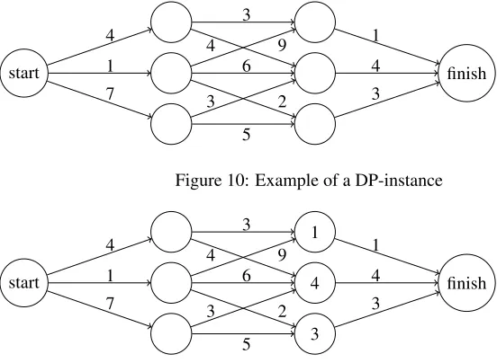
As an example, consider the shortest path problem in Figure 10. The goal here is to find the shortest path in this directed graph from start to finish, where the lengths of the edges are given. We can see that this is a DP instance with four phases, sorted vertically, as every edge is directed to the right.
For the points neighbouring to the final node, i.e. points from which the final node can be reached, we can see that there is only one path to the exit, with distances 1, 4 and 3 respectively. These numbers can be filled in as valuesV(s)of the corresponding statess, as is done in Figure 11.
Now we can consider the states in the second phase. For this, we can use the recursion (22), but as this is a minimization problem, we have to take the minimum, i.e.:
V(s) = min d∈D(s)F
start 4 5 7 1 4 3 finish 4 1 7 3 5 6 4 9 3 2 1 4 3
Figure 12: Example of a DP-instance; step 2
start 4 5 7 1 4 3 finish 4 1 7 3 5 6 4 9 3 2 1 4 3
Figure 13: Example of a DP-instance; optimal solution
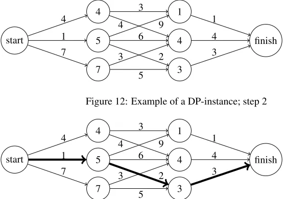
For the top-most state in the phase, we can see there are two possible decisions: the top one corresponds to a path length of 3 leading to a state of value 1, and the second decision has length 4 and leads to a state with value 4. As the revenues in this situation are the path lengths, we find that the value of the examined state is equal to min(3+1,4+4) =min(4,8) =4, which corresponds to the top-most decision.
Doing the same for the middle state, we find a value of min(9+1,6+4,2+3) =
min(10,10,5) =5, and for the bottom state we have min(3+4,5+4) =min(7,9) =7. Filling in these values leads to Figure 12.
Now the value of the initial state can be found, which is equal to min(4+4,1+
5,7+7) =min(8,6,14) =6. Therefore, the shortest path has length 6, and by track-ing back through the optimal solution and looktrack-ing which decision corresponded to the minimum path length, we can see the optimal path of the original problem is the path shown in Figure 13. This value could also have been found by starting from the ”start” node, and keeping track of the minimal cost to reach each state. This is known as ”for-ward Dynamic Programming”, while the technique we discussed is called ”back”for-ward Dynamic Programming”. Our ADP approach is most similar to backward Dynamic Programming, which is why it was discussed here.
3.2
The taxicab problem
heightnand widthm.
We call the position the taxicab startss0and the exit, the place the taxicab has to go
to,se. We define a path as a sequence of adjacent accessible grid points[s0,s1, ...,se]. Hence, a path is a way for the taxicab to reach the exit. The number of grid positions in such a path minus one is called the path length. We can see that the number of steps required for the taxicab is equal to the path length.
We can write this problem as a Dynamic Programming problem as follows: let the state space consist of the accessible points on the grid. For each statesletV(s)be equal to the minimum distance which is needed to get from pointsto the exit. Of course, for the exit this distance is 0. For the points adjacent to the exit, the distance is 1, and for the points bordering those points the distance is 2 (except for the exit itself of course). Continuing this process results in algorithm 1 to solve the taxicab problem with DP:
Algorithm 1Solve the taxicab problem using DP SetV(se) =0, setn:=0 andV(s) =m·n∀s6=se. Set listL:= [se]
whileV(s0) =m·ndo
setn:=n+1
for allstatessin L (i.e. all states that satisfyV(s) =n−1)do setV(s0):=nfor all neighbourss0ofsfor whichV(s0)>n add the statess0toL∗
end for
L:=L∗;L∗:=0/ end while
One can easily verify that in stepn this algorithm finds all the points at distance nfrom the exit point, so when the starting point is reached, the shortest distance from start to exit is known. The complexity of this approach is ofO(m·n), as each point is handled at most once. The number of neighbours is at most 4 for every state, so the complexity of handling a node is constant. This algorithm solves the problem quite satisfactorily, but ifmandnbecome large, it may not be too useful to search in every possible direction, but to instead search more towards the direction where the exit is situated.
3.3
ADP for the taxicab problem
In this subsection we attempt to solve the taxicab problem with Approximate Dynamic Programming. The aim here is to find a method that searches for a path to the exit, by repeatedly selecting steps that they are more likely to bring the taxicab closer to the exit. If the grid is not too complex, i.e. there are only few or no infeasible points, the shortest path has lengthO(max(m,n)), as the Manhattan distance between the starting point and the exit is at mostm+n. The ADP path is found step by step, where executing a step takes a constant time. Therefore, if the length of the path found is of the same order as the shortest path, we can see that the ADP algorithm finds this path inO(max(m,n))
After a path has been found, using an algorithm discussed later in this paragraph, the information on this path is used to improve on this path. We do this by looking back along the path to see which improvements were found. If we do thisktimes (where kmin(m,n)), this method should finish ink·O(max(m,n))O(m·n)time. We can see that this method indeed promises to give results faster, at the cost of losing certainty of finding an optimal solution.
In the next subsection we first explain how the value function works, and is updated once a path has been found. Then it is described how a path is found, whereby the value function is one of the factors used to determine the path.
3.3.1 Updating the value function
The base of the search for a path in this approach is a probability distribution over the possible directions for a given state. The idea is that we give ’better’ directions a higher probability. This probability distribution depends partly on known value estima-tions found from previous paths. The concrete way how a given path influences these decisions is presented in the following. In this subsection we assume that a path from start to exit has been found, and describe how the value function is updated.
Instead of the actual distance to the exit (which is unknown here), we use the min-imal distance we have encountered in previous paths, ˜V(s). Therefore ˜V(s)is always an upper bound for the valueV(s)of states.
Since the minimum distance can never be more than the number of grid points on the grid, we initialize ˜V(s)as follows:
˜ V(s) =
0 ifs=se m·n ifs6=se
(24)
Now, once a path to the exit(s0,s1, ...,sk−1,sk), wheresk=se, has been found, we track back along this path. In every statesi, we then update the values ˜V(s)for a state in the pathsiby taking the minimum of the current minimum path length ˜V(s)and the path created by first moving to statesi+1and then taking the shortest path from there.
As this path has length has ˜V(si+1) +1, the value function can be updated by setting:
˜
V(si):=min(V˜(si+1) +1,V˜(si)) (25)
for states{sk−1,sk−2, ...,s2,s1}.
3.3.2 Finding the path
In this subsection it is explained how a new path is found. We first define the set of possible directions ¯D:={up,down,le f t,right}. Before taking a step, for every possible directiond∈D¯ a probability to walk in that direction is determined. Then, a realization of this probability distribution determines the direction of the next step in the path. In the implemented algorithm we have chosen to let the probability depend on the following measures:
• not going back: if the taxicab goes back to the grid point it just came from, it is likely that no new information is obtained. Therefore, the probability of returning to the previous point is made smaller.
• forward consistency: To prevent small cycles, which do not add a lot of informa-tion, we give a bonus to the probability that the direction is in the same direction as the previous step.
• the minimum distance found so far (i.e. the value ˜V(si)for the different points siadjacent to the current position of the taxicab): Paths with a lower value have been found to result in shorter paths, so these states are more likely to be used in a path of shorter length.
We now translate these measures into numbers, depending respectively on param-etersA,B,CandD, which are fixed model parameters. These parameters describe the importance of each measure, and are used as follows:
A(s,d) =
Aif the Manhattan distance to the exit is decreased
0 otherwise (26)
B(s,d) =
Bifdis in the opposite direction of the previous step
0 otherwise (27)
C(s,d) =
Cifdfollows the same direction as the previous step
0 otherwise (28)
D(s,d) =
Dif ˜V(Tr(s,d))is minimal for alld∈D¯ and ˜V((Tr(s,d))<m·n 0 otherwise
(29)
Note that the last condition in D(s,d)makes sure that D(s,d) =0 if the value of all neighbouring states ofs equals the initial value, as that indicates there is no information about the distance to the exit. A positive value forD(s,d)in this situation would therefore only increase the randomness of the algorithm, which is not desired. For the other variables it is simply checked whether the desired feature is present. If it is, the corresponding variable gets valueA,B,CorD.
These variables are used to define the probability score. This is a nonnegative number that is calculated for every allowed direction, and is used to find the actual probability of walking in a certain direction. For the probability scorePS(d)we have chosen the following formula for every possible directiond∈D:¯
PS(s,d) =
K+A(s,d)−B(s,d) +C(s,d) +D(s,d) ifdleads to an allowed point
0 otherwise
In choosing these parameters, we should always ensure that PS(s,d)≥0 for all d∈D¯ and that ∑d∈¯
DPS(s,d)>0. This makes sure that we can indeed rescale the scores to probabilities. Ifdis a direction that leads to an inaccessible point, or crosses the edge of the grid, we setPS(d) =0.
From these probability scores we now define the probability of going to direction d,P(s,d), as follows:
P(s,d):= PS(s,d)
∑i∈D¯PS(s,i)
(31)
This gives a probability distribution over the different possible directionsd ∈D,¯ from which we can take a realization to choose a direction for the next step. This probability distribution is largely determined by the parametersA,B,C,DandK. We could split these parameters into 3 groups; the global steering variablesAandD, where Ais a parameter that steers the path to a closer Manhattan distance to the exit, and Dlooks at the results from previous paths. BandC can be considered consistency parameters, that ensure the path does not contain too many turns (B) and loops (C).K is a parameter that determines the randomness of the algorithm, or the influence of the steering of the other variables.
This method leads to an iteration of the grid as given by algorithm 2. During such an iteration also the value function ˜V(s)is updated.
Algorithm 2Calibration of ˜V(s)with a sample path s←s0, pathp←[s0]
whilese∈/ pdo
FindP(s,d)for all directionsdfrom statesas described in (31) Generate a directiondfrom this probability distribution AddTr(s,d)to the pathp: p←[p,Tr(s,d)]
s←Tr(s,d)
end while
UpdateV(s)as described in (25)
This algorithm is repeatedktimes in order to find a better estimate for the value function.
3.4
Results and analysis
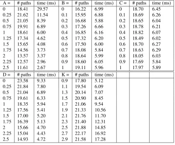
In order to see if this algorithm works, and how we should choose the parameters, this algorithm is applied to different grids. We have chosen the default values of this algorithm atA=1,B=0.9,C=0.3,D=1 andK=1.
A = # paths time (ms) B = # paths time (ms) C = # paths time (ms)
0 18.41 29.57 0 16.22 6.99 0 18.70 6.45
0.25 21.62 11.54 0.1 15.95 6.88 0.1 18.69 6.26
0.5 21.05 8.39 0.2 16.68 5.88 0.2 18.65 6.04
0.75 19.91 6.89 0.3 17.26 6.66 0.3 18.78 6.21
1 18.61 6.00 0.4 16.85 6.16 0.4 18.82 6.07
1.25 17.34 4.62 0.5 17.32 6.20 0.5 18.49 6.02
1.5 15.65 4.08 0.6 17.50 6.00 0.6 18.70 6.27
1.75 14.56 3.73 0.7 18.08 5.84 0.7 18.63 6.29
2 13.57 3.37 0.8 18.64 5.99 0.8 18.05 6.03
2.25 12.57 2.96 0.9 18.60 6.05 0.9 17.69 5.84
2.5 11.61 2.67 1 19.11 5.96 1 17.97 5.89
D = # paths time (ms) K = # paths time (ms)
0 23.58 9.33 0.9 17.80 5.12
0.25 21.84 7.80 1.1 19.54 6.09 0.5 21.04 6.89 1.3 20.14 7.07 0.75 19.61 6.33 1.5 20.90 8.45
1 18.35 5.94 1.7 21.06 9.54
1.25 17.56 5.41 1.9 21.33 10.56 1.5 17.00 5.20 2.1 21.76 11.70 1.75 16.39 5.13 2.3 21.40 12.31
2 15.66 4.70 2.5 21.88 14.85
[image:28.612.134.492.243.539.2]2.25 15.04 4.43 2.7 22.17 16.92 2.5 14.93 4.72 2.9 21.58 17.28
3.4.1 Grid 1
First of all, we consider a 50 x 50 grid with no obstacles, where the start (red) is the top left corner, and the exit (green) in the bottom right corner, as shown in Figure 14. The presented algorithm was applied to this grid. We ran this algorithm until the optimal solution of 98 steps was found, and then we looked at which iteration this optimum was found, and the time it took to find this optimal solution. As the directions are chosen randomly in this algorithm, a different run can have a different result. Therefore, we decided to restart the algorithm a total of 1,000 times for each combination of values. The average values found in these runs are shown in Table 1.
Examining the effect of a change in the parameterA, we see that larger values lead to a decrease of the time needed to find the optimal solution. The reason for this is fairly obvious, as in this empty grid every step toward the exit is an optimal step. So if Aincreases, the probability of taking an optimal step increases, and an optimal solution is found faster. The number of paths needed also decreases asAis increased, with the exception of small values ofA(0≤A≤0.5). This can be explained by the fact that a smallerAleads to longer paths, which contain more information. Hence, as expected, a largerAmakes the algorithm faster and in general it takes less paths to find the optimal solution.
ForB, we see that ifBbecomes larger, the number of paths increases while the time needed to find the optimal solution decreases. This indicates that for higher values ofB the paths are shorter, but because the longer, ’worse’ paths contain more information, less of these paths are required. But taking the time as an indication of the quality of the algorithm, we see that larger values forBproduces better results for this grid.
ForCwe see that both the number of the iterations the optimal solution was found in and the running time do not show much difference, but both seem to show a decreasing trend. This indicates that the optimal solution is computed slightly faster and uses less paths asCtakes larger values.
IfDis increased the required number of paths decreases, as well as the running time. AsDincreases, the focus is more about improving the previous paths than it is to find more or less new paths. As in this grid most non-optimal paths can be made optimal by finding a few shortcuts, improving previous paths is quite a good strategy, which explains this result.
ForK we picked a minimum value of 0.9, because a lower K could cause proba-bilitiesP(s,d)to become negative. Here we see that the more random the algorithm becomes, the slower it finds the optimal paths. This is because the grid contains no inaccessible squares, and so the steering variablesA, B,CandDall have a positive effect on the algorithm, because of the considerations described above. Therefore, for this grid we can conclude that the lower the random factor is, the better the algorithm works.
3.4.2 Grid 2
A = sols avg sol best sol B = sols avg sol best sol C = sols avg sol best sol
0 200 98 98 0 67 116.1 98 0 67 121.2 102
0.25 200 98 98 0.1 80 116.8 100 0.1 72 117.8 100
0.5 183 100.1 98 0.2 87 114.1 100 0.2 89 121.7 98
0.75 133 107.3 98 0.3 76 116.6 100 0.3 79 119.3 100
1 88 117.7 100 0.4 83 117.2 98 0.4 91 116.7 100
1.25 53 123.8 100 0.5 81 116.8 100 0.5 102 118.6 98
1.5 41 124.6 108 0.6 80 116.3 98 0.6 112 117.4 98
1.75 13 123.5 112 0.7 87 120.0 98 0.7 115 114.9 98
2 12 127.5 110 0.8 92 119.8 100 0.8 116 114.7 98
2.25 19 121.1 112 0.9 88 118.3 98 0.9 131 113.8 98
2.5 13 123.1 108 1 77 123.1 100 1 147 113.8 98
D = sols avg sol best sol K = sols avg sol best sol
0 87 136.2 112 0.9 80 119.5 98
0.25 68 132.6 108 1.1 110 116.0 98
0.5 80 128.2 104 1.3 122 115.2 98
0.75 91 126.8 102 1.5 139 112.7 98
1 80 118.6 100 1.7 157 109.1 98
1.25 79 114.1 98 1.9 174 108.7 98
1.5 84 110.1 98 2.1 175 107.0 98
1.75 92 107.6 98 2.3 186 106.5 98
2 80 106.8 98 2.5 184 103.6 98
2.25 83 105.6 98 2.7 191 102.3 98
[image:31.612.135.560.240.535.2]2.5 86 105.8 98 2.9 199 99.1 98
down. We have run the algorithm on this grid as well, but only used 200 runs, as more time was needed for this grid. Here it was found that here the optimum solution was not always reached. In fact, often no solution was found at all in 200 iterations, after which the algorithm was stopped. This is because the algorithm has to find the narrow bridge over the block, for which the variableAturned out to have very bad influence, as the algorithm is pulled the path on the region left to the bottom of the block, as the minimum distance to the exit reaches a local minimum there. For this reason the average solution after 200 iterations in 200 runs (avg sol) is shown. The average is taken only over the values where a solution was found, runs without a solution were not considered in finding the ’avg sol’-value. We also show the best solution found (bestsol), and the amount of runs in which in a solution was found at all (sol). The result of the simulation can be found in Table 2.
We see that the algorithm for this grid runs better for a smaller value ofA. This is, as mentioned before, due to the fact that initially the path is pulled towards the region left to the bottom of the block, as there is a local minimum value for the distance there. As the path keeps being pulled there, it becomes very hard to leave that region.
Looking at the performance of the algorithm whenBis changed, we see that the algorithm produces quite consistent results, so it seems that this variable doesn’t have a lot of effect in this case.
For parameterC, we can observe that the algorithm seems to get better whenCis increased. This can easily be seen from the number of times a solution is found, and also from the average final solution. This can be explained not only by less cycles in the algorithm, but also because a straight line is needed in large part of the optimal solution.
ForD, we see that the algorithm gets better asDbecomes larger. An explanation for this is that once a path to the exit has been found, the path is pulled towards this path, and more and better solutions can be found from there. Also, as D takes larger values, the presence of the ”bad” variable A becomes less important.
Looking at K, we can observe that the algorithm gets better as the randomness factor increases. When the algorithm is more random, there is less pull to the region to the left to the bottom of the block, and so the algorithm has a better chance of finding the bridge over the block. This causes more solutions to be found, and the final solution to be better.
3.4.3 Grid 3
For the third grid we inserted some blocks of unaccessible squares on the grid, leading to the grid in Figure 16. It can be easily verified that there is a solution of length 98, which uses a long horizontal line in the middle of the grid.
Looking at the different values ofA, we see that the solution gets worse whileA takes larger values. The reason for this is that a larger value ofAcreates a diagonal pull to the finish, where the optimal solution requires partly a horizontal line in the middle. AsAgets larger, it also becomes harder to get back to this horizontal line once it drops below. We also see that the algorithm initially become faster asAbecomes larger, but if it gets too large, the taxicab tends to get caught behind the little vertical block near the exit, and so the algorithm becomes slower for higher values ofA.
AsBtakes larger values, we see that the time it takes to solve the problem decreases, while the average solution seems to get a little bit worse. This is explained by the fact that decreasing the probability of going back makes it harder to return to the short horizontal path, but does create shorter paths, so it takes less time.
IncreasingCleads to better solutions, and also the time needed to find the solution decreases. This is because the optimal solution uses a long horizontal line, which is of course easier discovered when the probability of continuing in the same direction is increases. Also, a higherCleads to more consistent paths, so once the path is going in the right direction, it is more likely to keep going there. Of course, this also holds when the path is going in the wrong direction, but apparently this is outweighed by the positive effects, causing the solving speed to increase as well.
WhenDis increased we see that the quality of the result of the algorithm becomes worse. This is not too surprising, as the first time it is likely that the algorithm does not find an optimal algorithm, and after that it is drawn to that path, which makes it harder to deviate and find the optimal path. A largerD does lead to faster solving times, because the algorithm is more likely to follow the previous path and thus typically has no problem to find the exit.
ForK, a higherK implies more randomness, which increases the probability of finding the optimal solution. It also gives the best result over all changes we tried. This is explained by the fact that a higherK causes longer runs, which contain more information. Also, with a higherKthe path is not too much disturbed by the diagonal pull direction ofA, and the pull towards (non-optimal) previous paths ofD. Of course, a higherKalso increases the average number of steps needed to find the exit, which results in a longer running time.
3.5
Conclusion
The approximate dynamic program presented in this section seems to provide reason-able solutions for solving the taxicab problem. The program was run under different parameters for several different grids, and for each grid the optimal solution was found for at least some parameter configurations. Different parameters often provided differ-ent results, which were all fairly intuitive and could easily be explained, and often even predicted. So we have indeed managed to solve some instances of the taxicab problem with Approximate Dynamic Programming.
es-A = avg sol time (ms) B = avg sol time (ms) C = avg sol time (ms)
0 100.4 114.4 0 101.59 84.2 0 101.82 64.0
0.25 100.9 78.1 0.1 101.58 79.0 0.1 101.79 63.4 0.5 101.36 70.3 0.2 101.61 76.5 0.2 101.70 63.4 0.75 101.63 66.9 0.3 101.63 74.1 0.3 101.64 63.2 1 101.69 64.6 0.4 101.57 71.6 0.4 101.62 63.1 1.25 101.77 64.0 0.5 101.65 69.1 0.5 101.60 63.0 1.5 101.85 64.8 0.6 101.67 66.7 0.6 101.49 63.2 1.75 101.81 66.4 0.7 101.63 64.3 0.7 101.48 62.6 2 101.82 69.3 0.8 101.70 62.3 0.8 101.34 62.9 2.25 101.88 73.1 0.9 101.66 59.3 0.9 101.29 62.8
2.5 101.85 77.6 1 101.63 57.1 1 101.20 62.3
[image:35.612.135.491.244.540.2]D = avg sol time (ms) K = avg sol time (ms) 0 100.63 141.0 0.9 101.71 60.7 0.25 101.09 97.0 1.1 101.63 74.5 0.5 101.36 78.7 1.3 101.49 75.6 0.75 101.57 68.5 1.5 101.17 83.9 1 101.73 62.3 1.7 101.00 92.6 1.25 101.73 58.2 1.9 100.83 102.1 1.5 101.78 55.6 2.1 100.50 111.2 1.75 101.80 52.8 2.3 100.24 120.8 2 101.80 51.1 2.5 99.84 130.4 2.25 101.78 49.5 2.7 99.62 140.1 2.5 101.83 48.6 2.9 99.34 150.7
timated values. We already saw that too much exploration takes more time and leads to less useful states being visited, while too much exploitation leads to too much rep-etition and worse solutions as we saw in grids 2 and 3. This is a dilemma already described in literature, see for example Powell [2] and James [3].
We also saw that multiple runs of the same algorithm (but with a different random seed) can lead to different results. Therefore, it seems to be a good idea to run the algorithm multiple times and take the best results, if it involves randomness. This often works better than trying new iterations from the previous values. We also have seen that the best choice of the parameter settings depends on the grid. So if it is necessary to estimate some parameters in the model, we need to be careful.
4
ADP Approach
In this section we present an Approximate Dynamic Programming approach to the micro-CHP problem presented in Section 2. This approach is slightly different from the approach to the taxicab problem. This is because in the micro-CHP problem there are too many states to store values for all of them. Keeping track of just the values of the states that are visited is also difficult, not only because this number can become too large as well, but also because it is difficult to look up the stored values, if not all are stored.
Therefore, instead of keeping track of values for all states, as we did for the taxicab problem, in this section an approximation of the value function is considered. In this approximation, we use features of the current state, where a feature uses some char-acteristics of a state, indicating something about its quality. Basis functions are used to transform these features into numerical values. To obtain an approximation for the value function of a state, we use a weighted sum of these basis functions. The weights used to scale the basis functions depend on the phase, so that every phasethas its own weights.
Although this method is quite different from the ADP approach in the previous section, there are a lot of similarities between the two applications of ADP, so that the experience from the previous section can still be used.
In this section first the decision space is reduced, as there are simply too many decisions from a state to consider all of them. Then the structure of the chosen value function is specified. In the final subsection we explain how the parameters of this value function are updated, using the values of the path found.
4.1
Reducing the decision space
In this subsection we will describe the way in which the decision space is reduced in our ADP approach. Currently, the decision vectord consists ofN binary decision variables, whereN is the number of houses. This means that for a typical instance of 100 houses at each state we have 2100≈1030possible decision vectors. This is of course too many to consider them all. To deal with this problem, we consider only a subset of the possible decisions.
To do this, we introduce in each state a strict priority list for the houses. For this the houses are ordered on a measure of suitability to beonin the next interval. Once this list is determined, the only allowed decisions are to take theondecision for the first houses on the priority list, and theoff decision is made for the remaining houses. Hereby the only decision that can be made is how many houses are turned on. In other words, we determinen, 0≤n≤N, after which theondecision is taken for the firstn houses on the priority list, and the other houses are turnedoff. As in this situation the only decision left is to determinen, the number of decisions is decreased from 2N to N+1. Of course, we also lose a lot of flexibility here.
of course very unsuited to beonin the next interval, so we imposeR(i):=∞. For the remaining houses,R(i)is defined as the number of consecutive intervals that the off-decision can be taken, without a constraint being violated. Note, that if theoff-decision cannot be taken in the next interval, so the only feasible decision is to turn the house on, we getR(i) =0, putting these houses in the front of the list. This is a desirable property, as these houses are of course the best suited to be turned on.
For the other houses, the idea is that a higher value ofR(i)leaves more options in the next intervals. If houseihasR(i) =1, and we decide to turn it off in the coming interval, we already know that it has to be turned on in the next interval. If we turn off a house for whichR(i) =2, we will likely have both theonand theoff decision available in the following interval (unless the off time constraint 4 prevents that). For a house withR(i) =3 it takes even longer to get a forced decision if it remains turned off, so that house receives less priority to be turned on.
We define ˜Das the set of decision vectors that can be obtained in this manner for n∈ {0,1, ...,N}. Note that we consider all possible values within this set in taking these decisions. This includes the decisions leading to an infeasibility, e.g. switching on a houseifor whichR(i) =∞or switching off a house for whichR(i) =0. We do this because in some cases, all decisions are infeasible, or lead to an infeasibility in the future, and we still need to make a decision in these cases.
4.2
The value function
In this subsection we describe how the value function is initiated and updated. As we have mentioned before, the number of visited states typically becomes too large to keep track of values for all of them, as we have done in solving the taxicab problem. There-fore, we estimate this value function by consideringFdifferent features that apply to any statest∈S. Then, features f ∈ {1,2, ...,F} are mapped to a number by a basis functionφf(st). A weighted sum of these basis functions is used to find an estimate of the value.
In this weighted sum, the basis functions are multiplied by the phase-dependent weight of the featureθf,t. These weights are updated after a decision from a state in phaset has been chosen, which means that all weights are updated once during each iteration. The set of weights at a certain time is denoted byθt:={θ1,t,θ2,t, ...,θF,t}.
In formula form, the approximate value function ˜V(st,θt)looks as follows:
˜
V(st,θt) =
∑
f∈Fθf,tφf(st) (32)
If these weights and basis functions work well, the approximate value of the reach-able states can be calculated, and these values can be used to find the best decision, according to this approximation.
The approximate value function we use here has the same interpretation asV(st) in Section 2: the maximum revenue from all future electricity sales being in statestat timet. For the final interval we infer ˜V(sT,θT):=0, as after the final time interval no more electricity is sold.
is violated, an amountPis subtracted from the total revenue if the global electricity constraint (7) is violated. If another constraint, e.g. the heat level constraint (6), is violated, an amount of 10Pis subtracted.Pwill be chosen in the order of the maximum total revenue that can be obtained by all houses in one time interval. This ensures that a feasible solution is always preferred over an infeasible solution.
This change is made because the obtained revenues of a found solution are used to update the weightsθf,t, and in this update values of−∞are very impractical. This becomes clear in the description of the method of updating the weights. Furthermore, we have chosen a smaller penalty when the global electricity constraint (7) is violated, so that in case of a choice of constraint violations, violation of constraint (7) takes preference. This will lead to an easier comparison between different infeasible runs, as often the same constraint is violated in these cases.
4.2.1 Value function decomposition
In this paragraph, the parameters and basis functions we have chosen to represent the value function are presented.
We have chosen to introduce four basis functions, so that the value function has the following form:
˜
V(st,θt) =θ1,tφ1(st) +θ2,tφ2(st) +θ3,tφ3(st) +θ4,tφ4(st) (33)
In the following each of these basis functions are defined and explained.
• φ1(st)is an estimate of the total maximum sales revenue of electricity from state
st. To obtain this, we drop the global electricity constraint, after which we look at each houseiindividually, and simplify the situation of the house. We assume that a house only produces when its micro-CHP is switched on, and that it produces the maximum electricityHmax in these intervals. This implies that to find the current heat level, the streak value ai,t and the number of on/off switches ci,t are not relevant anymore; only the total running timebi,t matters. Finally, all constraints are discarded as well, except for the heat level constraints (6) for the final intervalT, for all housesi. In this heavily simplified model, the number intervals where the micro-CHP of houseihas to be on is fixed for every house i, as this is the maximum number ofon-intervals such that the heat level after intervalT is within the heat bounds. If we denote this number of intervals byw, the maximum revenue can be obtained by turning the micro-CHP on during the wintervals in{t+1, ...,T}where the electricity price is the highest. This is done for all housesi, and the sum of these revenues is used as an estimate of the total sales revenue from statest.
• φ2(st)consists of the minimum total amount of penalties received for constraint
violations during intervalt+1. These penalties are the revenues of −P and
First we check all constraints but the global electricity constraint (7). This is done by looking for houses for which both theonandoffdecisions are infeasible. A penalty of 10Pis obtained for every house for which this holds.
To account for the global electricity constraint (7) we first find theR(i)-value for all houses, as we did in finding the optimal decisions. Then, we can find the min-imum total electricity generation in the next interval by choosing theoff-decision for all houses for whichR(i)>0, and theon-decision for the remaining houses. Obviously, this is the minimum electricity production that can be obtained in a feasible way. If this minimum value is higher than the upper electricity bound Emax, a penalty ofPis unavoidable, and will be considered inφ2(st). Similarly,
the maximum total electricity production is found by determining the electric-ity production obtained when all houses are assumedonwhenR(i)<∞, and this value is compared toEmin. Again, a penalty ofPis obtained if this value is lower.
• To calculateφ3(st)we first determine the number of houses for which both theon and theoffdecisions are feasible. To obtainφ3(st), this number is downscaled by multiplying this number withk3, a fixed model parameter, which is done to make
this basis function fit better to the size of the other basis functions. The idea here is that more houses with two possible decisions leads to more flexibility, which can be a useful property.
• Withφ4(st), we want to ensure that the average remaining electricity production is in line with EminandEmax. Otherwise, it could happen that a large part of the production takes place in the first part of the day, producing aroundEmax in every interval, leaving not enough room for electricity production later, so that Emincan not be reached.
To prevent this, we first find the average electricity production per time interval from timet on,Eavg, and compare that value to the minimum and maximum production in each interval. To calculateEmax, we first determine for every house ian estimate of the final electricity level after intervalT,Lf inal,i. This is a model parameter that lies between the heat bounds 0 andLmax,i, which tries to make an accurate prediction of the electricity level.
Then we determine for every houseithe numberZ(i), which indicates how much heat has to be produced to reach this level, also considering the heat demands and heat losses. This is summed over all the houses, to find an estimate of the remain-ing heat production. To convert this estimate into an estimate of the electricity production, we estimate that the ratio between electricity and heat production is approximately the ratio of their maxima. Therefore, we define the numberηas
Hmax
Emax, and divide by this number to convert the heat demand to electricity
produc-tion.Eavgcan now be found by dividing this number by the number of remaining intervalsT−t+1:
Eavg:=
∑Ni=1Z(i)
Eavgis compared with the upper and lower bounds for the total electricity duction. These differences are converted to a fraction of the maximum heat pro-duction by dividing byNHmax to obtain the relative difference from the bounds. To do this, we defineduanddlas follows:
du:=
η(Emax−Eavg)
NHmax
, dl:=
η(Eavg−Emin)
NHmax
(35)
Th