Generalized Statistical Means and New Price Index Formulas, Notes on some unexplored index formulas, their interpretations and generalizations

(1)

Generalized Statistical Means and New

Price Index Formulas, Notes on some

unexplored index formulas, their

interpretations and generalizations

von der Lippe, Peter

University of Duisburg-Essen, Germany

10 June 2015

Online at

https://mpra.ub.uni-muenchen.de/64952/

(2)

Notes on some unexplored index formulas, their interpretations and

generalizations

Peter von der Lippe

The theory of (increasingly more generalized types of) statistical means can be used to create a plethora of index formulas. Some of them are new and some were indeed discussed in the past but fallen into oblivion, because their rationale was not well understood. Surprisingly many possess interesting interpretations and attractive properties that deserve being unveiled. We begin with unweighted indices with implications to what now is called "low level aggre-gation" and proceed to weighted index formulas that lend themselves to productive generali-zations and thereby to some new formulas. It turns out that contrary to popular belief the Laspeyres and Paasche formula are not equally well justified and that some indices from the more comprehensive system of statistical means are attractive regarding their economic inter-pretation and how they are related to indices of "quantity" and purchasing power of money.

1. Unweighted indices (low level aggregation) 1 2.3 Index type: price and quantity index 9 1.1. Unweighted indices and implicit quantities 1 3. AOR part II: More about PHB and PPA 9 1.2. Crossing of formulas and weights 2 3.1. Price indices with constant expenditures 9 1.3. Index of Allyn A. Young 1923 (PY 3 3.2. Price indices as reciprocal quantity indices 10 2. Weighted indices: AOR* formulas part I 4 3.3. PL and PP are not equally justified indices 11 2.1. Fisher's system and Vogt's generalized

anti-harmonic mean 4

3.4. Axiomatic performance of PHB and PPA 12 4. Weighted indices: ROA** formulas 16 2.2. Power means (generalized means) and

prod-ucts of power means 8

Appendix 17

References 18

* Average of ratios formulas ** Ratios of averages

1. Unweighted indices (low level aggregation)

1.1. Unweighted indices and implicit quantities

Carli's index 



0 i it C

t 0

p p n 1

P was widely used in early price level measurement in the 19th cen-tury.1 It was considered desirable to account for the different relative "importance" of the n goods in this formula. However, difficulties with aggregating over widely different types of goods and their quantities2 (we cannot add kilograms of vegetables, liters of fuel, yards of cloth, hours of services etc) have led some authors to adopt the idea of reciprocal prices as "implicit quantities": obviously 1/pi0 is the amount of good i you get for one currency unit

(say 1€, or 1$) at the base period.3

With such "implicit quantities" a mean of price relatives becomes a ratio of expenditures. When exactly 1€ was spent for each good in the base period, we have a basket of n goods and an expenditure (or cost for a basket) of E0 = n€ in the base

period and Carli's index PC compares Et =



 





n 1 i

1 0 i it p

p with E0 =



p_i₀

 

p_i₀ 1n, because

1

Laspeyres and some other authors made extensively use of this formula, then also known as "Sauerbeck index" in these days, and of Sauerbeck's price statistics for the British foreign trade. It was only in the 20th

century owing to Walsh 1901 that it became generally known that the formula actually was much older and originated from Gian Rinaldo Carli (1720 -1795).

2

A problem inherent in unit-value-indices (see below part 4)

3

Note reciprocal prices are not quantities. Just as a price is measured in currency units per unit of the quantity in

(3)

(1.1)



      

 

0 i

it n

1 0 i it n 1 0 i it

0 t C

t 0

p p n 1 n

p 1 p

n p

1 p

E E

P .

It may also be interpreted as comparing weighted average prices (with reciprocal prices or implicit quantities as weights), p Et n

C

t  and p E0 n 1

C

0   . With this (admittedly

some-what farfetched) notion of "implicit quantities" an average of price ratios (or AOR-formula) can easily be translated into a ratio of average expenditures/prices or ROA formula. Or in other words: an unweighted index may be viewed as implicitly, i.e. with reciprocal prices weighted. The same logic, if applied to an unweighted harmonic mean will lead to

(1.2)

 

*

0 * t 1 it 0 i

1 it it

it 0 i 1

1

0 i

it n

1 H

t 0

E E p

p p p p

p n p

p

P _   

  

  

      





 



where E*_t and E*₀ are expenditures

with current period "implicit quantities" 1p_it . That P₀H_t 

 

P_tC₀ 1means that PH is the "time antithesis" (as Fisher would have put it) of PC (and vice versa). Note that using relative prices or "price shares" (or price quotas p/p) rather than reciprocal prices we also can transform a ROA type index such as Dutot's index PD into a weighted AOR index like of the PC or PH type

0 t 0 i n 1

it n 1 0 i it D

t 0

p p p p p

p

P   



as weighted (PC-type) AOR index 



i0

0 i 0 i it D

t 0

p p p p

P and

0 t 1

it 0 i D

t 0

p p p

p P _ 

  

   





_ 1

it it it

0 i D

t 0

p p p p P



    

  



 

as weighted PH type AOR index.4

ROA form weights AOR form

ratio of average ex-penditures/prices* as for example PD

relative prices p/p average of price ratios

[= price relatives] as for example PC and P H

reciprocal prices (as implicit quantities)

* equal implicit quantities 1/n for each good

Obviously in (1.1) and (1.2) the "quantity" of each good is indirectly proportional to its price, so expensive goods are less, and cheaper goods are more represented in such an index. This suggests taking some average of such implicit quantity weights (leading to Young's index PY).

The formulas PC (Carli) and PH (harmonic) were mainly discussed (and rejected) because of

their failing the time reversal test since P_tC₀ 

   

P₀H_t 1 P₀C_t 1 and P_tH₀ 

   

P₀C_t 1 P₀H_t 1.

1.2. Crossing of formulas and weights

A quite natural idea is to take a mean of PC and PH. The geometric mean of PC and PH, that is

(1.3)





 

it 0 i

0 i it

it 0 i 0

i it H

t 0 C

t 0 CSWD

t 0

p p

p p n : p p n 1 P

P

P , is known as CSWD-index5 and

for approximating the time reversible index of Jevons n

0 i it J

t 0

p p

P 



. It can easily be seen that

4

So taking a harmonic mean of the price relatives with weights pit/pit will again yield PD. Unlike Carli's

(4)

PJ and PCSWD pass the time reversal test, since 1 P_tJ₀ P₀J_t P_tCSWD₀ 1 P₀CSWD_t .6 In a similar

man-ner we can also take averages of weights





i 0 i

i it CW

t 0

W p

P where the part of weights Wi can be

taken by

 A

p p

i

i it

  



 

 

1 2

1 1

0

(arithmetic) giving





i 0 i

i it )

A ( CW

t 0

A p

P _C

0 t

C t 0

P 1

  

 H

p p

i

i it

 

2

0

(harmonic), yielding





i 0 i

i it )

H ( CW

t 0

H p

P









 



 

p p p

it i it

i i it

/ ( )

0

0 0

, and







1 _i _i

it 0 i

i p p AH

G    (geometric) 





i 0 i

i it )

G ( CW

t 0

G p

P ₀Y_t

it 0 i

0 i it

P p / p

p / p

 



_.

In all three cases both, numerator pitWi and denominator pi0Wi may be viewed as expendi-tures, or (upon division by n) as weighted average prices. So crossed implicit weight (CW) indices can be given an ROA-interpretation in addition to an AOR interpretation as for

exam-ple











  

) p p /( p

) p p /( p p p

P

it 0 i 0 i

it 0 i 0 i 0 i

it )

H ( CW

t

0 is an average of price relatives pit/pi0. The most interesting

index is PCW(G) as it coincides with an index PY suggested by Allyn A. Young (1923)7.

1.3. Index of Allyn A. Young PY

Young proposed the following seemingly weird and unmotivated formula

(1.4)



 

t 0 0 t

t 0 0

t 0 t Y

t 0

p p p p

p p

1 p

p p

1 p

P

linear ho-mogeneity

time reversal test

yes no

yes Y C, H, CSWD

no CW(A), CW(H)

Given this favourable situation of PY the question may arise why this index did not find atten-tion and why it obviously is completely fallen into oblivion. We think that this is due to the fact that its rationale is not well understood when it was proposed in 1923.8 Nobody seems to know by which underlying "logic" (of crossing inverse prices as implicit quantities) we would arrive at Young's index PY. So some remarks to its rationale should be pertinent here:Young found that "base year weighting" in P₀C_t 



p_t

 

p₀ 1



p₀

 

p₀ 1 (with weights in the way of inverse base period prices or implicit quantities) tends to "overweight rising prices", while

5

As acronym for Carruthers, Selwood, Ward and Dalen.

6

PJ has both, an AOR and a ROA interpretation (taking geometric means of prices averages in the ROA).

7

This Young is not to confound with Arthur Young 1812, also often quoted in index theory literature. Unlike PCW(G) the formulas PCW(A) and PCW(H) possibly rightly did not receive much attention.

8

Irving Fisher 1927; 530f later called PY "an ingenious anomaly, scarcely classifiable" (in the scheme of Fisher's book) and "a scientific curiosity".

(5)

 

_

 



 

 1

t 0 1 t t H

t

0 p p p p

P , tends to underweight them. Thus he was quite naturally lead to

seek a compromise using the geometric mean

t 0p

p 1

. Later Bert Balk rediscovered Young's

formula and called it Balk-Walsh (BW) index, because with explicit (quantity) weights we get

Walsh's formula





t 0 0

t 0 t W

t 0

q q p

P which bears some resemblance to Young's formula PY

based on implicit (inverse prices) rather than explicit weights. Another rediscovery of PY took place when Jens Mehrhoff – in a short note he contributed to von der Lippe 2007; 45f – look-ing for a linear index able to approximate PCSWD and thereby PJ. He called it "hybrid" and later "BMW (Balk-Mehrhoff-Walsh) index", not knowing that it coincides with PY and he also remarked (like von Bortkiewicz and even already Young before), that PY not only has a ROA interpretation (indicated in (1.4) with weighted means of prices) but also an AOR inter-pretation as follows

(1.5)





t 0 t 0 0 t Y

t 0

p p p p p p

P ,

"In a way Professor Fisher is right in holding that all true index numbers are averages of ratios. But I should prefer to say that all true index numbers are at once averages of ratios and ratios of aggre-gates." (Young 1923; 359).

Young also saw that his index meets the time reversal test but not the circular test, because



 

2 1 1 2

1 0 0 1

2 0 0 2 Y

02

p p p p

P , and finally (interesting in view of Mehrhoff's paper) Young

also noted about PY "In general it will agree very closely with the geometric average" (357).

2. Weighted indices: Average of ratios formulas (AOR), part I:

2.1. Fisher's system and Vogt's generalized antiharmonic mean

A distinction can be made between first, second, and third order index formulas (Köves 1983; 28ff, v. d. Lippe 2007; 54). "First" means unweighted indices, "second" relates to Irving Fisher's system of AOR-formulas and "third" to "crossing" of second generation indices (for example Fisher's ideal index as result of crossing Laspeyres and Paasche). Fisher introduced

 sixtypes of (unweighted) means (of price relatives), of which only arithmetic, harmonic and geometric means are worth being considered,9 and

 fourmethods of weighting (I through IV, of which he called two, II and III "hybrid") by which he arrived at the following system:10

9

The three remaining means are median, mode, and the "aggregative" index as Fisher called it (like the Dutot index pt/p0). They are no longer of any interest.

10

Note that some of the combinations are identical due to inherent relations between the arithmetic and the har-monic mean: both index formulas, PL and PP can be expressed in two ways, using pure and hybrid weights. It will soon be shown that all the remaining indices can be written in two different ways as well (see tab. 3).

(6)

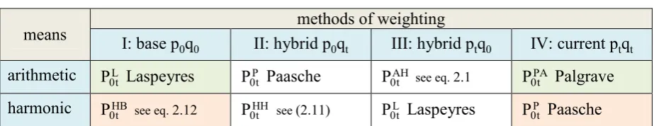
Table 1

means _{I: base p} methods of weighting

0q0 II: hybrid p0qt III: hybrid ptq0 IV: current ptqt

arithmetic PL_t

0 Laspeyres P0Pt Paasche P0AHt see eq. 2.1 P0PAt Palgrave

harmonic PHB_t

0 see eq. 2.12 P0HHt see (2.11) P0Lt Laspeyres P0Pt Paasche

The highlighting with green n orange color is meant as hint to related fields (in the same color) of table 2

The combination gives six different "second generation" index-formulas PL, PP, PAH, PPA, PHB, and PHH (of which only the indices of Laspeyres and Paasche are well known, PPA refers to the index of Palgrave, and the other labels are our own: HB = harmonic base, HH = harmonic hybrid, AH = arithmetic hybrid). The indices PHB and PPA are a bit more interesting than the indices PAH and PHH (which are rarely if ever seriously considered), so PHB and PPA will be discussed in more detail below (section 3).11

Obviously P0AHt is related to the so called quadratic mean (QM) as follows

(2.1)   



0 t

0 0 2 t 0

t 0 t 0 t AH

t 0

q p

p q p q

p q p p p

P





_L

t 0

2 QM

t 0 0

0 0 t

0 0 0 0 2 0 2 t

P ) P ( q

p q p

p p q p p p





where QM t 0

P is the quadratic and L t 0

P the arithmetic mean of price relatives with type I weights. The system of tab. 1 can be generalized in view of

 the fact that all means, harmonic (x_H) geometric (x ) arithmetic ( x ) and quadratic _G (x_QM) are special cases of x r_p

 

, the power mean (moment mean or generalized mean) of degree r given by

(2.2)



m rm



1/r

r 2 2 r 1 1

P(r) wx +w x +...+w x

x  ,12 and

 the (weighted) antiharmonic mean (denoted by H to avoid confusion with AH denot-ing arithmetic hybrid) of x-values with weights w discussed in Vogt 1979

(2.3)





i i

i 2 i H

w x

x =

 

x_Q 2 x

[image:6.595.71.533.85.174.2]

that is the ratio of the squared quadratic and the arithmetic mean,13 so that PAH is in fact an antiharmonic mean using weights of type I. This motivates an extension of the scheme above as follows:

Table 1a

mean _{I: base p} methods of weighting

0q0 II: hybrid p0qt III: hybrid ptq0 IV: current ptqt

antiharmonic P₀AH_t P₀GAH_t

 

0,1 PA t 0 2 H

t 0 P

P  P₀H_t3 (2.10) P₀H_t4 P₀GAH_t

 

t,1

11

In Germany Neubauer 1998 brought them into play and v. d. Lippe 2000 discussed their properties.

12

The special cases are r = -1 harmonic mean, r  0 geometric mean, r = 1 the arithmetic mean and r = 2 quad-ratic mean. According to a corollary, first proven by Cramer the power mean is a monotonous function in the parameter r such that harmonic  geometric  arithmetic  quadratic (equality applies when all x-values are identical). From this follows PHH < PP < PPA and PHB < PL < PAH in tab. 1

13

(7)

 the even more general concept of the generalized antiharmonic or "GAH" mean

(again brought into play by Vogt)

(2.4)



     





k

0 t j

1 k

0 t j GAH

t 0

p p s

p p s ) k , j (

P

[image:7.595.64.525.217.299.2]

and the GAH mean allows some interesting extensions of table 1.

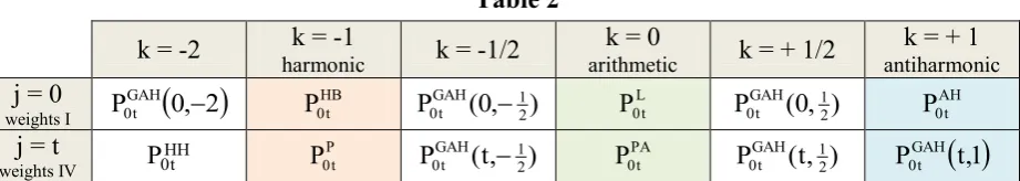
Table 2

k = -2 k = -1

harmonic k = -1/2

k = 0

arithmetic k = + 1/2

k = + 1

antiharmonic

j = 0

weights I P



0, 2



GAH t 0 

HB t 0

P PGAH(0, ₂1)

t 0 

L t 0

P PGAH(0,₂1)

t 0

AH t 0

P

j = t

weights IV Pt

HH 0

P t 0

P PGAH(t, ₂1)

t 0 

PA t 0

P PGAH(t,₂1)

t

0 P

 

t,1 GAH

t 0

In table 2 there are no longer any hybrid weights Together with two additional rows for hybrid weights (type II and III) we would get with k = -1 (orange) and k = 0 (green) the complete table 1 as a special case (subset) of table 2.

[image:7.595.65.392.369.621.2]

Before going into details of table 1a and 2 it may be useful to introduce certain fictitious quantities in the following table

Table 1b

deflated inflated

q0

t 0 0 0 t

0 D 0

p p q p p

q q  

0 t 0 I 0

p p q q 

qt

t 0 t 0 t

t D t

p p q p p

q q  

0 t t I t

p p q q 

The missing formula P₀H_t2 in tab. 1a now is

(2.9)



 

_



t t

I t t

t 0

t 0 0 t

t 0

t 0 2 0 2 t 2

H t 0

q p

q p q

p q p p p

q p

q p p p

P = PA

t 0

P and for H3 t 0

P we get

(2.10)

 





) q p (

q p p p

P _I

0 t

I 0 t 0 t 3

H t 0

which does not seem to be a useful formula. This also applies to PHH which is given by

(2.11)



 _D

t 0

t 0 HH

t 0

q p

P , or written as a GAH (t, -2) index



 

     



t t 2

0 t

t t 1

0 t HH

t 0

q p p p

P

which bears some resemblance with

with expenditure shares sij = pijqij/pijqij (j = 0, t, hybrid "weights" will henceforth no longer be con-sidered; summation takes place over i) taking the place of the weights wi above.

k = 1 is the "usual" antiharmonic mean introduced above.

The red double arrow means I t

q is the "time antithesis" (I. Fisher) of qD₀ (and vice versa), and so is D

t

q of I 0

q . We will come back to this table 1b in section 3 in our attempt to give a meaningful interpretation to HB

t 0

P and PA t 0

(8)

(2.12)



 _D 0 0 0 0 HB t 0 q p q p

P , or written as a GAH (0, -1) index



              0 0 1 0 t 0 0 0 0 t HB t 0 q p p p q p p p P .

From tab. 2 two remaining formulas may be of some interest:

) 2 , 0 ( P0GAHt 











t

D 0 0 0 t D 0 0 t p q p p p q p

p _{harmonic mean weights} D

0 0q

p

(deflated base period)

) 1 , t ( PGAH t 0











0

I t t t 0 0 I t t t p q p p p q p

p _{arithmetic mean weights} I

t tq

p

(inflated current period)

Surprisingly: while the indices PAH and PHH were introduced already above as indices with hybrid weights, it turns out now in tab. 2 that they also emerge as indices with "pure" weights I and IV. So types of means and types of weights are somehow related. As to the still remaining four indices of tab. 2:

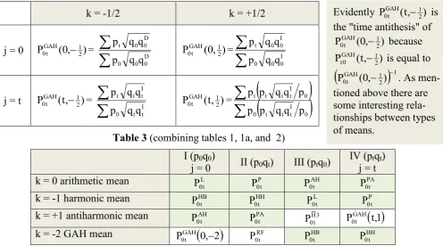
k = -1/2 k = +1/2

j = 0 PGAH(0, ₂1)

t

0  =



D

0 0 0 D 0 0 t q q p q q p ) , 0 ( PGAH ₂1

t

0 =



I

0 0 0 I 0 0 t q q p q q p

j = t PGAH(t, ₂1)

t

0  =



I

t t 0 I t t t q q p q q p ) , t ( PGAH ₂1

t

0 =











0

I t t t 0 0 I t t t t p q q p p p q q p p

Table 3 (combining tables 1, 1a, and 2)

I (p0q0)

j = 0 II (p0qt) III (ptq0)

IV (ptqt) j = t

k = 0 arithmetic mean L

t 0

P P₀P_t P₀AH_t P₀PA_t

k = -1 harmonic mean HB

t 0 P HH t 0 P L t 0 P P t 0 P

k = +1 antiharmonic mean AH

t 0

P PA t 0

P H3 t 0

P PGAH

 

t,1

t 0

k = -2 GAH mean _PGAH



₀_, ₂



t 0 

RF t 0

P P₀HB_t P₀HH_t

The four white fields represent indices of little or no use. We presented above the relevant formulas for three of them. The remaining formula (RF) reads as follows

 



 D t 0 t 0 D t 0 RF t 0 q p p p q p

P . Note that each of the six (more or less) meaningful index functions of

table 1 appears twice in the green fields. We now can offer a list of indices and their "time antitheses". Table 4 shows that we have six pairs:

Table 4

L t 0

P  P ₀P_t P₀HB_t  P₀PA_t PHH_t 0 

AH t 0

P H3

t 0

P  P₀RF_t cp. table 7

) 2 , 0 (

P₀GAH_t   P₀GAH_t (t,1)P₀H_t4 PGAH(t, ₂1)

t

0   P (0, 2) 1 GAH

t

0 

In order to compare this with tab. 1 note that

AH t 0

P = P₀GAH_t

 

0,1 and

HH t 0

P = P₀GAH_t



t,2



Evidently PGAH(t, ₂1)

t

0  is

the "time antithesis" of )

, 0 ( PGAH ₂1

t

0  because

) , t ( PGAH ₂1

0

t  is equal to





1

2 1 GAH

t

0 (0, )

P   . As

[image:8.595.65.562.295.571.2]

(9)

From the above formula for P₀AH_t follows P₀AH_t P₀L_t and P₀HH_t P₀P_t,14 and as P₀HH_t is the "time antithesis" of P₀AH_t the index P₀AH_t P₀HH_t as well as P₀PA_t P₀HB_t follow the model of Fisher's ide-al index F 

t 0 P P t 0 L t 0 P

P . About this more below.15

We now are also able to classify unweighted – i.e. weights of s = 1/n – price index formulas

using the unweighted GAH formula



_

         

  k

0 t 1 k 0 t p p p p

for various values of k

Table 5

k - 1 - ½ 0 + ½ 1

formula harmo-nic PH

Young PY

using (1.4) Carli P C



0 t 0 t 0 t p p p p p p



0 t 0 t 0 t p p p p p p

The Fisher like index (geometric mean of an index and its time antithesis) is now is the CSWD index (PCPH)1/2 (as the unweighted analogon to PF).

2.2. Power means (generalized means) and products of power means

Power means (PM) of order r weighted with expenditure shares s allow to construct new in-dex functions and to demonstrate interesting relationships between existing inin-dex functions. The rth PM of price relatives with expenditure shares si0 = pi0qi0/ pi0qi0 is P₀PM_t (r,s₀) is given

by r / 1 i 2 r 0 i it 0 i 0 PM t 0 p p s ) s , r ( P              





. For r = 2 we have P₀PM_t (2,s₀)=

2 / 1 i 2 2 0 i it 0 i p p s              



= P₀L_t ,

and P (r,st)

PM t

0 for r = -2 (weights sit = pitqit/pitqit) is =

2 / 1 i 2 2 0 i it it t PM t 0 p p s ) s , 2 ( P                 



 = P t 0

P . This gives rise to study products of powermeans,

(2.13) P (r,s0)

PM t

0 P ( r,st) PM

t

0  =

r / 1 r / 1 i 2 r 0 i it it i 2 r 0 i it 0 i p p s p p s                              



 ,

of which – as demonstrated – Fisher's ideal index P₀L_tP₀P_t is the special case r = 2. 16 And r= -2 gives PPM( 2,s₀)

t

0  P ( ( 2),st) PM

t

0   =

PA t 0 HB t 0 P

P . Another case is r = 1

) s , 1 ( P₀PM_t  _t



 t 0 t t 0 0 0 0 t t 0 PM t 0 p p q p p q q p q p ) s , 1 (

P = V₀_t Q₀W_t P~₀W_t that is the "indirect" Walsh price index (ratio of value index and Walsh quantity index).17

14

To exceed PL (PAH > PL) or fall short of PP is of course not attractive. By contrast to be smaller than Laspeyres makes PHB attractive, and accordingly PPA > PP may be seen as an advantage of Palgrave's index.

15

It turns out that most of the Fisher-type indices formed with one of the eight pairs above are nonsensical.

16

The unweighted variant of this with sit = si0 = 1/n for all i is of course the CSWD index. 17

(10)

[image:10.595.63.577.411.655.2]

Table 6

A = PPM(r,s₀)

t

0 B = P ( r,st) PM

t

0  B* = P (r,st)

PM t

0 A* = P ( r,s0)

PM t 0  r / 1 i 2 r 0 i it 0 i p p s              



r / 1 i 2 r 0 i it it p p s               



 r / 1 i 2 r 0 i it it p p s              



r / 1 i 2 r 0 i it 0 i p p s               





1 



q₀ p₀p_t



q₀p₀ 



qtpt



qt p0pt  

2 _ L

t 0

P  P0Pt  

-1 _

_

D

0 0 0 D 0

tq p qq

p 



p_t q_tqI_t



p_oqI_t  

-2 _ HB

t 0

P  PA

t 0

P  

Obviously B is the "time antithesis" of A (and B* of A*) so that AB or A*B* is a Fisher-type index. Note also that  and  cannot be viewed as price indices because prices pt in the numerator and p0 in the denominator are not multiplied by the

same factor. The same is true for  and .

2.3. Index type: price and quantity index

The convention is that a price index is a ratio in which numerator and denominator differ with respect to prices but not quantities. The opposite applies to a quantity index: numerator and denominator are different regarding quantities, not prices. However, the divide between a price index on the one hand and a quantity index on the other becomes a bit blurred once we introduce fictitious (deflated or inflated) quantities

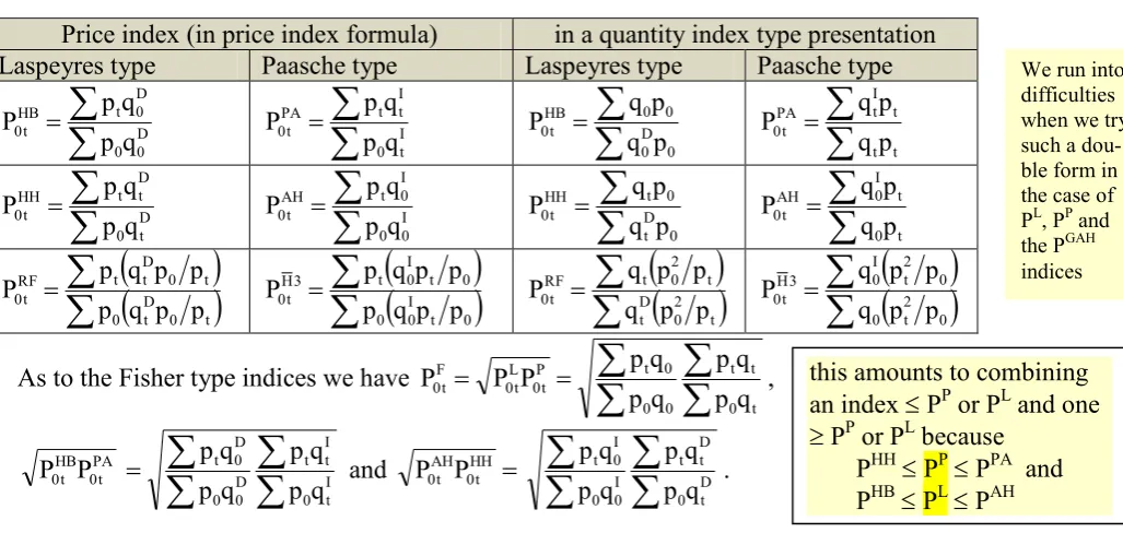
Table 7

Price index (in price index formula) in a quantity index type presentation

Laspeyres type Paasche type Laspeyres type Paasche type



 _D 0 0 D 0 t HB t 0 q p q p P



 _I t 0 I t t PA t 0 q p q p P



 0 D 0 0 0 HB t 0 p q p q P



 t t t I t PA t 0 p q p q P



 _D t 0 D t t HH t 0 q p q p P



 _I 0 0 I 0 t AH t 0 q p q p P



 0 D t 0 t HH t 0 p q p q P



 t 0 t I 0 AH t 0 p q p q P











 t 0 D t 0 t 0 D t t RF t 0 p p q p p p q p

P



_



_



 0 t I 0 0 0 t I 0 t 3 H t 0 p p q p p p q p

P



_



_



 t 2 0 D t t 2 0 t RF t 0 p p q p p q

P



_



_



 0 2 t 0 0 2 t I 0 3 H t 0 p p q p p q P

As to the Fisher type indices we have



  t 0 t t 0 0 0 t P t 0 L t 0 F t 0 q p q p q p q p P P P , PA t 0 HB t 0 P P



 _I t 0 I t t D 0 0 D 0 t q p q p q p q p

and P₀AH_t P₀HH_t 



D t 0 D t t I 0 0 I 0 t q p q p q p q p .

3. Average of ratios formulas (AOR), part II:

More about the weighted harmonic mean index (PHB) und Palgrave's index (PPA)

3.1. Price indices with constant expenditures

The following interpretation of PHB an PPA was brought into play in Germany by Werner Neubauer18: The rationale of the two rather unfamiliar indices PHB and PPA can be explained

18

I (and possibly Neubauer too) did not know that much of the following was seen already by W. Ferger.

We run into difficulties when we try such a dou-ble form in the case of PL, PP and the PGAH indices

this amounts to combining an index  PP or PL and one

(11)

using the fictitious quantities introduced in table 1b. The quantity q that is D₀ q_iD₀ q_i₀



p_i₀/p_it



in (2.12) 



D

0 0 0 0 HB

t

0 p q p q

P must be regarded as quantity you can afford under the re-gime of new prices pit ( D

0

q applies to period t) when you keep your expenditure (instead of the quantity) of period 0 constant for each commodity i, so that qD₀p_it p_i₀q_i₀ and therefore



D _it  _i₀ _i₀

0p p q

q . The meaning of inflation now is: the price level is rising to the extent to which we get less quantity for the same amount of money. With rising prices it = pit/pi0 > 1 follows from D _i₀ _i₀ _i₀ _it

0

i p p q

q   so that D _i₀

0 i q

q  holds for each commodity, and



D 0 0 i q

p <



pi0qi0for all commodities (not to confound with







i0 i0

D 0

itq p q

p ). To interpret the products D

0 tq

p and I t 0q

[image:11.595.67.533.291.460.2]

p is easy (as they are equal to p0q0 and ptqt respective-ly), but p₀qD₀ and p_tqI_t does not seem to be meaningful. However, with  >1 one can conclude

Table 8

fictitious vs. real quantities

fictitious vs. real expenditures (interpretation)

price index

the underlying perspective of the interpretation

D 0

q refers to t

 D ₀ 0 q

q 



D ₀ ₀

0

0q p q

p had I bought

in 0 (prices p0) the smaller quan-tity D

0

q (the one I can still afford in t) it had cost less than p0q0.

1 P₀HB_t 

to know and make use of qD₀ in t so that



D

0 itq

p = pi0qi0 requires to remember in t the expenditure of 0 (pi0qi0) I

t

q refers to 0

 I _t t q

q 



I  _t _t

t

tq pq

p if I would buy

in t the larger quantity I could have bought in 0 (with prices p0 < pt) it

would cost more now, in t

PA t 0

P >1

to know and make use of qI_t in 0 so that



p_i₀qI_it = pitqit requires to know in 0 the future

expenditure of t (pitqit)

To remember in t what we used to spend in 0 in order to adjust q0 so that D 0

q



qD₀p_it 



p_i₀q_i₀ is clearly a more realistic perspective than to transform q0 to q so that we now (in 0) with cur-I_t rent prices p0 spend the same amount of money we are going to spend in the future (with pric-es pt and quantitipric-es qt). So we have again the situation that the implicit thought experiment with PPA is more doubtful that in the case of PHB just like the underlying logic of PP is not on an equal footing with PL (as is generally believed) but clearly less stringent.

3.2. Price indices as reciprocal quantity indices

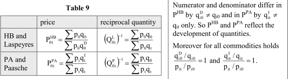
It is interesting to see what becomes apparent when we contrast PHB and PPA to reciprocal quantity indices of Laspeyres and Paasche:

Table 9

price reciprocal quantity

HB and

Laspeyres



 _D

0 0

0 0 HB

t 0

q p

P

 







t 0

0 0 1

L t 0

q p

q p Q

PA and

Paasche





t t

I t t PA

t 0

q p

P

 







t t

0 t 1

P t 0

q p

q p Q

Numerator and denominator differ in PHB by q D_i₀  qi0 and in PPA by q I_it  qit only. So PHB and PPA reflect the development of quantities.

Moreover for all commodities holds

1 p / p

q / q

0 i it

0 i D

0

i  _and ₁

p / p

q / q

0 i it

it I

[image:11.595.70.540.614.743.2]

(12)

Hence P₀HB_t and P₀PA_t may also be viewed as a reciprocal quantity indices using fictitious

quan-tities. The ratios on 1

p / q

p / q p / p

q / q

0 i 0 i

it D

0 i 0 i it

0 i D

0

i   _{and equivalently} ₁

p / p

q / q

0 i it

it I

it  _{may be viewed as}

(ra-tios) of elasticities. The "inverse quantity index" interpretation of a price index PHB or PPA is in line with the concept of inflation (as mentioned above) according to which a price level is rising to the extent to which we get less quantity for the same amount of money. It is also in harmony with reciprocal prices as fictitious quantities in the early index theory.

Not only PHB and PPA, also the Laspeyres and Paasche price index can be given an appearance of a reciprocal quantity index, because we have 



D

0 t 0 t L

t

0 pq pq

P and P

t 0

P =



0 t

I t

0q p q

p as counterparts of P₀HB_t 



p₀q₀



p₀q₀D and P₀PA_t 



p_tqI_t



p_tq_t. In Ferger 1931 a correctly developed theory can be found about when to use the weighted

(weights wi where w = wi) arithmetic mean _i

ixiw

w 1

x



as opposed to the harmonic mean

i i

i 1

H w

x 1 w

1 ) x

(  



. Ferger realized that x_H should be used when the task is to average rati-os

i i i

d n

x  where the numerator is constant (ni = n i) while x is the correct average, when the denominator is constant (di = d i) so that xi is a linear transformation of ni.19 Prices are by their very nature always ratios20 pi = ti/mi = expenditure for good i (monetary transac-tion)/mass (quantity of good i). So a household might be aiming to procure a constant (given) quantity, say m = q0 (to keep base period q0 constant (in whichcase PL would be appropriate) or to maintain the (base period) expenditure constant.21 And to our surprise on p. 40 we found

the formula of "our" indexP₀HB_t derived as weighted harmonic mean

1

0 0

0 0 t 0 HB

t 0

q p

q p p p P



    

  



 

.

We will come back to Ferger and thus to another interpretation of PHB in a short annex below.

3.3. Again Laspeyres (PL) and Paasche (PP) are not equally well reasoned indices22

Hence PL is related to PHB and so is PP to PPA. However, as noted already in sec. 3.1 to inter-pret PPA seems less straightforward than PHB, because I

it

q appears more fictitious than D 0 i

q . To argue in terms of q (based on future quantities qit) for a fictitious base period expenditure (as I_t in PPA) is much less plausible, than to introduce quantities D

0 i

q for the future based on

19

The "classic" example is velocities vi = Di/Ti= distance/time (i = 1,…,m) of m bikers. When all m bikers have

the same distanced to travel, so that they differ with respect to their elapsed time T1, …,Tm the harmonic mean

H

v is to be taken; while the arithmetic mean v would be correct when the winner is the one who covered the longest distance in a given time T. So a ratio can be viewed from different perspectives, and in PL and PHB simp-ly prices are viewed from different perspectives, both reasonable and legitimate.

20

This point was also (and at great length) made by Allyn Young 1921. We use the symbols t and m Young introduced, ti instead of piqi for the expenditure and mi instead of qi for the quantity (and t rather than q0). 21

Ferger discussed in detail which approach (orientation at quantities or at expenditures) would reflect more realistically the decisions of households, and he found that constancy of quantities q0 should be ruled out because

it would imply a zero price elasticity of demand. He explicitly derived PHB which he recommended for use, but he did not discuss how PHB is related to PL and that PL would be a kind of arithmetic analogon to the harmonic PHB. Interestingly and most noteworthy: he already saw that PHB vs. PL boils down to constant expenditures vs. constant quantities. So he already was aware of an interpretation Neubauer some thirty years later rediscovered.

22

(13)

ties qi0 of the past (as in PHB). It makes sense to ask: what can we consume in the future in order to keep to the expenditure of the past period 0, however, it is much less sensible to ask what we could have consumed in the past when we spent the same amount of money we do now, that is in the future period t (aiming at spending or imagining an expenditure amounting to p_i₀qI_it p_itq_itinthe past as in PP or in PPA – where PPA is even less rational because in PPA we recourse in a fictitious quantity I

t

q - is less realistic a problem than spending now, in t the sum qD₀ pt as we actually did in the past, when we spent q0p0). So we have here with PPA and PHB the same asymmetric relation as with PP and PL which shows once more, that PP and PL are – contrary to a common preoccupation – not equally reasonable index functions. There is a significant difference between these two indices that can easily be seen when one compares

the sequence ,...

q p

q p P

, q p

q p P

, q p

q p P

0 0

0 3 L

03 0 0

0 2 L

02 0 0

0 1 L

01



 

 where subsequent indices differ

only with respect to prices in the numerator, however in , q p

q p P

1 0

1 1 P

01





,... q p

q p P

, q p

q p P

3 0

3 3 P

03 2 0

2 2 P

02







also with constantly changing quantities in numerator and

denominator so that the elements P01, P02, P03, … in the sequence of prices indices are not comparable among themselves (what evidently applies to PHB and PPA too).

3.4. Axiomatic performance of PHB and PPA

Due to the relationship between arithmetic and harmonic means P₀HB_t < L t 0

P and P₀PA_t > P t 0

P . This may be welcomed as a valuable property of PHB and PPA, because it is often said that Paasche understates and Laspeyres overstates inflation as measured by a true price index: the

interval HB

t 0 TRUE

t 0 PA

t

0 P P

P   is smaller than L

t 0 TRUE

t 0 P

t

0 P P

P   . In this sense it also might be somewhat attractive to consider the time reversible price index PA

t 0 HB

t 0 P

P , built analogously to P₀F_t  P P₀L_t ₀P_t although an economic interpretation of this index must be challenging. Both indices, PHB and PPA are weakly monotonous, however, PPA is strictly monotonous only in the base period prices and PHB in the current period prices. Though all indices of table 1 are means of price relatives, that is they possess the mean value property M, only few of them, viz PL and PP are linear (= additive): Additivity (linearity) L is defined in table 10b and nei-ther PPA nor PHB satisfy both conditions of additivity.23 Property L is a subset of property M

23

Other examples of price indices which clearly are means of price relatives but nonetheless not linear are the logarithmic Laspeyres (also called geometric Laspeyres) price index DPL where ln(DPL) is the arithmetic mean of logarithmic price relatives (weighted with expenditure shares of the base period p0q0/p0q0), or the quadratic

mean of price relatives PQM.

M

L

M

(14)

Palgrave's index 



_t _t



_t _t

0 t PA

t

0 pq pq

p p

P is not linear (additive) in current period prices because this would require for p*_t = p_t+p_t to hold that



_













  _ 

   

 

 



 _t _t _t _t _t

0 t t t

0 t t *

t PA

t

0 p p q p q

p q p p

p q p )

(

P p is equal to

the sum of 



t



t t

0 t t t

PA t

0 p p q

p q p ) (

P p and









  _

t t t

0 t t t

PA t

0 p p q

p q p ) (

P p .

Table 10(a)

price index

HB t 0

P (harmonic base) P₀PA_t (Palgrave)

bounds HB

t 0

P < L t 0

P P

t 0

P < PA t 0

P

monotonicity*

weak monotonicity fulfilled by both indices, PHB and PPA PPAstrictly monotonous only in the base period prices, PHB is strictly monotonous only in current period prices

additivity not in base period prices not in current period prices aggregative

con-sistency (AC) both indices,

HB t 0

P and P₀PA_t are aggregative consistent

quantity indices both indices fail the factor reversal test and the indirect (implicit) quantity indices violate the proportionality axiom Q~₀_t  although qit = qi0 i * the reason for failing monotonicity is that p*_t p_t_{affects in P}PA_{both, price relatives}_and

weights (in PHB, however, only price relatives). The opposite applies to PHB that meets strict monotonicity only in current period prices but not in base period prices).

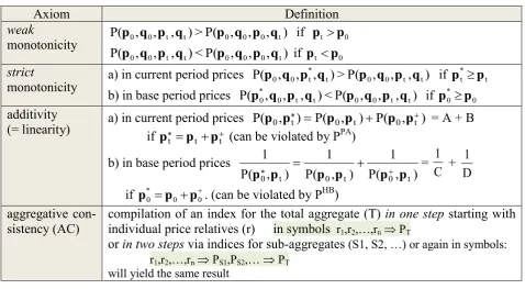
Table 10(b)

Axiom Definition

weak

monotonicity P( 0, 0, t, t)>P( 0, 0, 0, t)

q p q p q

p q

p if pt p0

) , , , P( < ) , , , (

P p₀ q₀ p_t q_t p₀ q₀ p₀ q_t if p_t p₀

strict

monotonicity

a) in current period prices P( , , *, _t)>P( ₀, ₀, _t, _t)

t 0

0 q p q p q p q

p if * _t

t p

p 

b) in base period prices P(p₀*,q₀,p_t,q_t)<P(p₀,q₀,p_t,q_t) if p*₀ p₀

additivity

(= linearity) a) in current period prices P( , t) P( , t) P( , t )

*

p p₀  p p₀  p p₀  = A + B if p*_t

t t

_p _p_{(can be violated by P}PA )

b) in base period prices 1 1 1

0 0 0

P(p p*, t) P(p p, t) P(p p, t)

 

 =

1 C +

1 D

if  0 0 *

0 p p

p . (can be violated by PHB) aggregative

con-sistency (AC)

compilation of an index for the total aggregate (T) in one step starting with individual price relatives (r) in symbols r1,r2,…,rn PT

or in two steps via indices for sub-aggregates (S1, S2, …) or again in symbols: r1,r2,…,rn PS1,PS2,…  PT

[image:14.595.69.548.72.423.2] [image:14.595.70.549.474.737.2]

(15)

It can easily be seen that PPA not even complies with linearity in the restricted case of p+_t 

  

 

  

  

b ...

b

b which means that "if all prices are increased by the same amount, the index of the

new prices should equal to the old index number plus the index number of the constant amount".24 A price index formula that complies with additivity (linearity) in both, base period

and current period prices can also be written as P₀_t t 0

 a p

b p '

' , that is as ratio of scalar vector

products.25 For example P₀L_t implies a' b'q₀' [constant], in P₀P_t we have a' b' q_t'. But

P₀HB_t and P₀PA_t though both means of price relatives are yet not additive (linear) functions in prices p0 and pt. Though we can write (see table 7)



 _D

0 0

D 0 t HB

t 0

q p

P and



 _I

t 0

I t t PA

t 0

q p

P this is

not in line with ' ₀

t ' t 0

P ap bp because unlike a and b the "quantity" vectors here (with ele-ments qI_t q_t(p_t p₀) and qD₀ q₀(p₀ p_t) respectively) are not independent of pt and p0.

Aside: The presentation in table 7 is particularly useful to relate these indices to linear in-dices. However the forms P₀PA_t 



p_tqI_t



p_tq_t and P₀HB_t 



p₀q₀



p₀q₀Dare better in order to demonstrate that under normal conditions of rising prices the indices exceed unity because then t

I t q

q  and 0

D 0 q

q  .

Just like linearity or additivity (L) and the mean value (of price relatives) indices (M) and should be kept distinct so also additivity (L) aggregative consistency (AC or simply C). How-ever, while L is a subset of M the situation with L and C is different

In the case of PHB and K = 2 sub-aggregates AC means that when the index for the total ag-gregate can be compiled in one step, say as harmonic mean of price relatives, the correspond-ing two step procedure via compilcorrespond-ing indices for K sub-aggregates which are subsequently aggregated (again as harmonic mean of the K sub-indices with base year expenditure weights) to the total index we should get the same result. It can easily be seen that indeed for K = 2 sub-aggregates, A and B, the total index P0HBt is a harmonic mean of P (A)

HB t

0 and P (B) HB

t 0

 

_



_

_



_

  

    

   

   



0 0

0 B 0 B 0

B 0 B

0 B 0 B Bt

0 B 0

0 0 A 0 A 0

A 0 A

0 A 0 A At

0 A 1

HB t 0

q p

q p q

p q p p p q

p q p q

p q p p p

P

24

Pfouts 1966 p. 176 also noticed that the famous "ideal" index PF of Fisher does not satisfy additivity (in all variants) either, not even in the restricted case above b' = [b b … b]. His paper was a sort of pamphlet against the (unmerited) prestige of the "ideal" Fisher index PF, an index he thought, should be abandoned.

25

von der Lippe 2007, 193. C L

CL (for example PL, PP),

C-L (PPA,PHB) so that PHB and PPA meet C though not L

for L-C an example is



0Pt



L

t 0 2

1 _P _P _{which is linear but}

vio-lates C because the weights ½ are not related to expenditure shares; and finally for

(16)









B 1 HB

t 0 A 1 HB

t

0 (A) g P (B) g

P   

 , with 1

q p

q p q

p q p g

g

0 0

0 B 0 B 0

0 0 A 0 A B

A  







 .

26

Other important properties of PHB and PPA concern quantity indices of the HB and PA type. A distinction has to be made between

 direct quantity indices Q0t gained from price indices P0t by interchanging prices and

quantities so that ₀ ₀

t 0 0

0 HB

t

0 p q

q q q

p

Q 



and 



_t _t



_t _t

0 t PA

t

0 pq pq

q q

Q , and

 indirect (implicit) quantity indices resulting from dividing the value index V0t =

ptqt/p0q0 by the respective price index Q~₀_t V₀_t P₀_t. Unlike the direct quantity indices HB

t 0

Q and PA t 0

Q the respective implicit quantity indices, that

is HB

t 0 t 0 HB

t

0 V P

Q~  and PA

t 0 t 0 PA

t

0 V P

Q~  will violate proportionality in the quantities and conse-quently also identity, This clearly invalidates them as deflators.27 The products PA0t

PA t 0 Q

P A

and BP₀HB_t QHB₀_t are in general unequal (A  B) and also different from the value index V0t, that is the indices of the HB and PA type are not factor reversible.28 Lack of proportionality of

HB t 0

Q~ QHB₀_t and Q~₀PA_t QPA₀_t (and thus a fortiori lack of identity),29 can easily be verified as follows: if q_it q_i₀ i then also  L 

t 0 P

t 0 Q

Q and therefore the indirect quantity indices will in general be Q~₀_t  because Q~₀HB_t = V0t/P₀HB_t = O₀PP₀L_t/P₀HB_t O₀LP₀P_t/P₀HB_t  unless

L t 0 P

t 0 HB

t

0 P P

P   . The same consideration leads to Q~PA₀_t . More specifically we can conclude

P t 0 HB

t

0 Q

~

Q~  because PL > PHB and Q~₀PA_t .

It is difficult to say something about how P₀HB_t P₀PA_t =



I

t 0

I t t D t 0

D t t

q p

q p q p

q p

differs from P₀F_t=

P t 0 L

t 0 P

P =



0 t

t t 0 0

0 t

q p

q p q p

q p

because it is the structure of weights that matters and nothing

definite can be said about how the structure of weights in PL vs. PHB and in PP vs. PPA differs:





0 0

0 0 0 t 0

0 0 t L

t 0

q p

q p p p q p

q p

P =



 

 _D

0 0

D 0 0 0 t HB

t 0

q p

q p p p A P

A and





t 0

t 0 0

t P

t 0

q p

q p p p

P =



 _I

t 0

I t 0 0 t PA

t 0

q p

q p p p P

B 1

. It is difficult make conclusions about A/B.

26

It can easily be verified that the corresponding equation (with arithmetic means) holds for PPA, so that also Palgrave's index is additively consistent.

27

When all quantities remain constant ( = 1), then using PHB as deflator would not result in V/PHB = 1 unless also all prices would remain constant (because then we have V=PHB = 1). Otherwise V/PHB shows (counterfactu-ally) a rising volume (and the deflator PPA analogously a decreasing volume).

28

Factor reversibility (the factor reversal test) amounts to equality of the direct and the indirect quantity index. Unlike the pair L/P (Laspeyres/Paasche), the pair HB/PA does not even pass the less demanding product-test.

29

(17)

4. Weighted indices: Ratios of averages formulas (ROA)

Many index functions possess both forms (formulas), an AOR form like 



0 i 0 i

0 i 0 i 0 i

it L

t 0

q p

q p p p P

with weights p_i₀q_i₀



p_i₀q_i₀ and a ROA form P₀L_t 



p_itq_i₀



p_i₀q_i₀ in which both numera-tor and denominanumera-tor reflect expenditure or average prices if divided by a suitable quantity. We encountered indices with an AOR form and an unfamiliar ROA form with no or only an at best far fetched AOR interpretation.30 To give only one example for an "ROA-only" index (with no AOR interpretation) we briefly mention Drobisch's index as ratio of a sort of abso-lute (e.g. expressed in $) price levels P~_t and P~₀ as "macro level" or (universal) "unit values" (3.1)



_



it it it it

it it t

q q p q

q p P

~

and P~₀ defined correspondingly, we get

(3.2) _D

01 t 0 it

0 i iß 0 i

it it 0

t DR

t 0

Q V q q q

p q p P

~P ~

P    



with Dutot's quantity index it i0

D t

0 q Q

Q 



. One of the problems with DR

t 0

P is that the sum over all goods and services is generally not defined (the summation fails already for the simple reason that there are quite different meas-uring units for the quantities). So as a rule DR

t 0

P cannot be compiled on the level of a national economy. This infeasible P₀DR_t is often called "unit value index"(UVI) and it is often con-founded with another indeed existing (in particular in foreign trade statistics where we have since long the habit to report quantities of exported or imported goods) UVI index, compiled with unit values (a sort of average prices) as building blocs instead of prices as building blocs. Assume the k-th aggregate can be decomposed into Jk individual goods j = 1,2,…,Jk. then its

unit value in t is ~ =p_kt

kt jkt jkt j jkt

j jkt jkt

q q p q

q

p



_

and in 0

0 k

0 jk 0 jk 0

k

q q p p

~ _



_,31

so that a Laspeyres

type (L) or (more commonly in use) Paasche (P) type unit value index can be compiled as

 



 



k j jk0 jk0 k j jkt jk0 L

t 0 k k0 k0 k kt k0 )

L ( UV

t 0

q p

q p P

q p ~

P and





k k0 kt k kt kt )

P ( UV

t 0

q p ~

q p ~ P

 

 

k j jk0 jkt k j jkt jkt P

t 0

q p

P .

Both indices evidently differ from DR t 0

P .32 The present author has repeatedly published papers explaining the difference between unit value indices P₀UV_t (L)and P₀UV_t (P) and genuine price indi-ces L

t 0

P and P t 0

P . There may be other "ROA-only" indices in addition to DR t 0

P , but it seems questionable that it is worthwhile discussing them. In von der Lippe (2013) we gave mention to a rather strange index formula of Lehr which is another example (in addition to PDR) for an "ROA-only" index.

Appendix: Ferger's index of purchasing power (PP)

According to Ferger an appropriate measure of the purchasing power (PP) of money is "not the reciprocal of an index of prices but an index of the reciprocals of prices properly

30

This applies to indices making use of fictitious quantities. There are of course also indices that possess none of the two forms, neither AOR nor ROA, for example Fisher's ideal index PF.

31

Unlike the overall sum of quantities kjqjkt and qjkt the k-specific qkt =jqjkt and qk0 can be compiled. 32

(18)

weighted" Ferger 1936, p 266 (Ferger's emphasis). As an unweighted version of such an index

of reciprocal prices Prp he studied

 

H

t H 0 1 H 0

1 H t

0 i n 1

it n 1

p p p

p p

1 p

1



 _





, and he demonstrated33 the

differ-erence between his Prp concept and the ruling "macro" PP concept as reciprocal price index

(P-1), with the example

 

t 0 1 D

t 0

p p

P   . The reason why he rejected this P-1 approach of inverting a price index was, that he opposed the then (in the "stochastic index theory") popular idea of a hidden general driving force that makes all prices increase or decrease more or less in uni-son.34 So he thought a measure of PP should address individual prices as a sort of "micro" approach35 and consider expenditures rather than quantities.36 Ferger realizeded that the dif-ference between his favoured index H

t H 0 p

p and the P-1 approach using

 

D 1 ₀ _t t

0 p p

P  

"arises from the different weights applied by the formula despite our proposed intention of maintain-ing equal weights. The price index gives more weight to the price of the expensive article A by as-suming constant quantities to be bought, while the purchasing power index gives more weight to the price change of the cheaper article B by assuming constant expenditure to be maintained" (268).

For a weighted index of PP (i.e. of reciprocal prices) Ferger considered expenditures e0 = pi0qi0, but such weights need an adjustment because what we get for 1$ and thus for e0$

de-pends on the prices. So weights should be 2 _i₀ 0 i 0 i

0 i 0

i ₍_p ₎ _q

p 1

q

p _

and it can easily be seen that













HB

t 0 0

0 t 0 0 0 0

i 2 0 i 0 i

0 i 2 0 i it

P 1 q

p p p q p q

) p ( p 1

q ) p ( p 1

 



and





PA

t 0 it 2 it 0 i

it 2 it it

P 1 q ) p ( p 1

q ) p ( p 1





. Division by 1/pi0 or

1/pit means that expenditure is not measured in $ but in units37 per $ which comes closer to a sort of standardized and dimensionless quantity.

As an aside: For Ferger's PP index (PHB)-1 but not for the price index PHB we have a time se-ries interpretation as we had in sec. 3.3 (p. 12 above) for the price index PL of Laspeyres

be-cause of the constant denominator







0 0

1 0 0 0

q p

p p q p

,







0 0

2 0 0 0

q p

p p q p

,







0 0

3 0 0 0

q p

p p q p

,… In

this respect the PP index (PPA)-1 is less attractive as (PHB)-1 just like PPA is short of PHB (or PP short of PL). Interestingly Ferger started out with the Prp idea but ended up with a P-1 type of

33

Using a numerical example, p. 267.

34

He also disapproved the preference (in the stochastic index theory) for unweighted indices which was based on the idea that each price relative was considered an independent representative of the same general force driving prices up or down. So Ferger was explicitly in favour of weighting with expenditure weights (we already noticed above his interesting interpretation of PHB in terms of keeping expenditures rather than quantities constant).

35

This is of course rather absurd: we cannot speak of a purchasing power of money with respect to cheese, shoes etc. but only of a purchasing power of a specified income spent for a bundle of clearly defined purchases. Not-withstanding his idea "There is no change in the value of money except that which is result of, or rather is com-posed of changes in the prices of commodities"(262f) is of course correct.

36

"If we are measuring changes in its [the money's] buying power over several commodities, we must thus measure the changing quantities of these commodities when the same amounts of money are paid for them re-spectively, rather than measuring the varying total cost of the same respective quantities" (Ferger 1936, p. 268).

37

Interestingly Fergers symbol for 1/p0 is u0 (u for "unit"). We already saw that 1/p0 or 1/pt may be viewed as