Stochastic conditonal range, a latent variable model for financial volatility

Munich Personal RePEc Archive

Stochastic conditonal range, a latent

variable model for financial volatility

Galli, Fausto

University of Salerno

28 February 2014

Stochastic conditional range, a latent variable model

for financial volatility

Fausto Galli

Abstract

In this paper we introduce a parameter driven model for the dynamics of range,

the stochastic conditional range (SCR). We propose to estimate its parameters by

Kalman filter, importance sampling and simulated maximum likelihood depending

on the hypotheses on the distributional form of the innovations. The model is applied

to a large subset of the S&P 500 components. A comparison with of its fitting and

forecasting abilities with the CARR model shows that the new approach can provide

an interesting alternative.

∗_{DISES and CELPE, University of Salerno. Address: Dipartimento di Scienze Economiche e Statistiche}

1

Introduction

It is a well known phenomenon that financial time series exhibit volatility clustering. A very large literature on the dynamics of returns has developed since the seminal contributions of Engle (1982), Bollerslev (1986) and Taylor (2007) on GARCH and stochastic volatility. Most of this literature concentrates on the dynamics of the differences of closing prices of the reference period as a means of describing the subtle concept of volatility.

Parkinson (1980) suggested that the use of extreme price values can provide a superior estimate of volatility than returns. The potential advantages of using price range as an alternative were also pointed out by Alizadeh, Brandt, and Diebold (2002), who claimed to “show theoretically, numerically, and empirically that range-based volatility proxies are not only highly efficient, but also approximately Gaussian and robust to microstructure noise”, while Brandt and Diebold (2006) noticed that range “is a highly efficient volatility proxy, distilling volatility information from the entire intraday price path, in contrast to volatility proxies based on the daily return, such as the daily squared return, which use only the opening and closing prices”.

Chou (2005) proposed a dynamic model, the conditional autoregressive range (CARR) for the evolution of high/low range who mimics the structure of the ACD model of Engle and Russell (1998) for inter trade durations. This line of modelling has desirable statistical and empirical properties and the search for its refinements and extensions can draw from the wide body of ACD literature.

one affecting the observed range and the other the latent variable. The model can be seen as characterized by a mixture of distribution, or, in following Cox (1981), as parameter-driven. This specification also shares most of the statistical characteristics of the stochastic conditional duration (SCD) model of Bauwens and Veredas (2004). In section 2, we will present the model and discuss some of its properties. In section 3 we propose three methods for estimation: maximum likelihood based on Kalman filter or on numerical integration of the latent variable and indirect inference. A comparison on the fitting and predictive capabilities of CARR and SCR models is carried out for a large sample of stocks in section 5. Results show that the SCR provides more reliable estimates of the autocorrelations of the data process, while in terms of forecasting accuracy it is comparable to CARR.

2

The model

Let pτ the price of a financial asset sampled at frequent (e.g. minutes or seconds) time

intervals τ, and Pτ = ln(pτ) its logarithm. We define as range the difference Rt =

max(Pt)−min(Pt), where t indicates a coarser set of time intervals (e.g. days, weeks)

such that

τ =t−1, t−1 + 1

n, t−1 +

2

n, . . . , t, (1)

wherenis the number of frequent intervals contained in one of the coarser intervals indexed byt.

The conditional autoregressive range CARR(1,1), introduced by Chou (2005) is defined by the following equations:

Rt= Ψtǫt (2)

with

ω >0, α≥0, β ≥0,

where the baseline range (the error) ǫt has a distribution with density functionp(ǫ), which

has positive support and unit mean. It denotes the information set at time t−1, and it

includes the past values of Rt and ψt.

Computing moments and autocorrelation for the CARR(1,1) model is easy and one can obtain the following simple expression:

E(Rt) =

ω

1−α−β if (α+β)<1, (4)

E(R2t) = E(Rt)2

1 +σ2

ǫ(1−β2−2αβ)

1−(α+β)2_−α2_σ2 ǫ

, (5)

ρ1 =

α(1−β2_−αβ)

1−β2_−2αβ , (6)

ρn= (α+β)ρn−₁ (n >1). (7)

We introduce the stochastic conditional range (SCR) as the process described by the following equations:

Rt=eψtǫt (8)

ψt=ω+βψt−1+σut (9)

where ut|It−₁ has an iid standard normal distribution and ǫ_t|I_t−₁ has, like in the case of

CARR, a distribution defined on the positive axis with unitary mean.

The expected value of the range conditional to the past of the process up to time t−1 is

E(Rt|It−₁) =e

ψt

and the distribution of ǫt. The condition |β| < 1 is necessary and sufficient to ensure

stationarity and ergodicity for the process ψt, and hence for Rt.

The theoretical first two moments and the s-th autocorrelation ofRt are the following

E(Rt) =E(ǫt)E(eψt) = e ω

1−β+

σ2

1−β2, (10)

E(R2t) =E(Rt)2

E(ǫ2 t)

E(ǫt)2

e σ

2 1−β2

−1

+E(Rt)2, (11)

ρs=

e

σ2_{ǫ β}s

1−β2 −1

E(ǫ2 t)e

σ2ǫ

1−β2 −1

(12)

for all s≥1.1

Concerning the distribution of ǫt, any law with positive support can be a suitable

candidate. In this paper we will use two distributions: the Weibull and the log-normal. Weibull distribution is commonly employed in duration analysis and was adopted by Chou (2005) in the CARR model. The justification for the use of the log-normal distribution arises from the result by Alizadeh, Brandt, and Diebold (2002) on the distribution of daily high and low prices, which appears to be approximately Gaussian. Depending on the choice of the distribution for ǫt, the estimated models will be denoted as W-SCR and L-SCR.

As it was noted above, we restrict the first moment of the baseline rangeǫtto be equal to

one. This is necessary to avoid an identification problem between the expectations ofǫtand

ψt. The location parameter of the log-normal distribution will be therefore set to −1/2σǫ2,

while the scale parameter of the Weibull will be restricted to be equal to Γ(1 + 1/γ)−1

, where σ2

ǫ and γ are the shape parameters which will be let free to vary.

1

3

Estimation

In this section we will discuss how the estimation of the SCR model can be performed either by maximum likelihood (ML) or by indirect inference.2 _{Concerning ML estimation,}

we will detail the methods that can be followed in order to deal with the problem of the presence of a latent variable.

3.1

ML with Kalman filter and EIS

The distribution of the baseline rangeǫtplays an important role in deciding how to proceed

in the computation of the likelihood function to be maximized.

If ǫt is log-normally distributed, as in the L-SCR specification, the model can be

trasformed by taking the logarithms on both sides of equation (8). This yields the fol-lowing relationships

rt= lnRt=ψt+ lnǫt, (13)

ψt=ω+βψt−1+σut, (14)

that can be interpreted as the state and transition equations of a linear state-space model. This model can be easily estimated by Kalman filter and the resulting likelihood can be maximized by means of a numerical algorithm.

The reliance of the Kalman filter on the normality of both error components (lnǫt

and ut) limits its use to the L-SCR case only. When the distribution of ǫt is exponential

or Weibull, the Kalman filter will not produce an efficient computation of the likelihood anymore.3 _{Therefore, it is necessary to resort to the numerical integration of the density}

2

In the literature on SCD models, which share the same functional form with SCR, some alternative approaches are explored. For example Knight and Ning (2008) compare two solutions based on GMM and on empirical characteristic function and Strickland, Forbes, and Martin (2006) follow a Bayesian approach based on MCMC integration of the latent variable.

3

of the latent variable to compute an exact likelihood.

To do this, we start by denoting by R a sequence ofn realizations of the range process.

R has a conditional density of g(R|ψ, θ1), where θ1 is a parameter vector indexing the

distribution andψ a vector of latent variables of the same dimension of the sampleR. The joint density of ψ is h(ψ|θ2), with θ2 a vector of parameters, and the likelihood function

for R can be written as

L(θ, R) =

Z

g(R|ψ, θ1)h(ψ|θ2)dψ=

Z n

Y

t=1

p(Rt|ψt, θ1)q(ψt|ψt−₁, θ₂)dψt (15)

the last term of the equation is the result of the sequential decomposition of the integrand in the product of the density of ǫt conditional on ψt, p(Rt|ψt, θ1), that in our case will be

Weibull, and the density of ψtconditional on its past, q(ψt|ψt−₁, θ₂), which is normal with

mean ω+βψt−₁ and variance σ2.

This high dimensional integral is not analytically solvable and a numerical approach is necessary. There is a very substantial literature on Monte Carlo integration methods, for an interesting survey in the field of stochastic volatility see Broto and Ruiz (2004).

The method we will employ is a refinement of the widespread importance sampling technique, it is called efficient importance sampling (EIS) and was developed by Richard and Zhang (2007). As the authors point out, this method is particularly convenient for an accurate numerical solution of high dimensional ”relatively simple” integrals like the ones we need to treat and has already been successfully applied to problems that are similar (see Liesenfeld and Richard (2003) and Bauwens and Hautsch (2006)) or nearly identical (see Bauwens and Galli (2009)) to ours.

For a detailed presentation of the algorithm, we refer the reader to Richard and Zhang

(2007). A description of its implementation in the contest of the SCD model, which share the same functional form with the model proposed in this paper is available in Bauwens and Galli (2009). In the appendix we present a brief summary.

3.2

Indirect inference

An alternative solution for the estimation of the parameters of the SCR models can consist in indirect inference (for a detailed introduction see Gouri´eroux and Monfort (1996)), a simulation-based method that can be useful in estimating models for which the likelihood function is difficult to evaluate. Indirect inference relies on the possibility of easily simulat-ing data from the model which is object of estimation (the estimand model). Simulations from the estimand are evaluated through a criterion function constructed with an approx-imate, or auxiliary, model, whose estimation can be performed easily (at least relatively to the estimand model). The auxiliary model does not necessarily provide an accurate de-scription of the true process that generated the data, working more as a window through which to view both the actual data and the ones simulated from the estimand model. The objective of indirect inference is to choose the parameters of the estimand model so that they minimize a distance between the results of the estimation (that can consist in the parameters, the likelihood or the score) of the auxiliary model with the simulate data and the actual ones. A brief summary of this method is presented in the appendix.

For the indirect inference estimation of the SCR model, we chose two auxiliary models: an AR(10) and an ARMA(1,1)4_{. Both models were estimated on the logarithm of the}

observed and simulated ranges. As a result of the estimation of the two auxiliary models we chose to use their parameters and a simple sum of their squared differences was employed as the distance to minimize to obtain the indirect inference estimator.

4

3.3

Estimation of the latent variables

Once estimates the parameters of the models have been obtained, it is possible to compute estimates of the latent variable ψt. The process described by equations 13 and 14 is in the

form of a linear state space model, and this allows to employ Bayesian updating in order to recover estimates for a prediction step, that provides a one-step-ahead prediction of the latent variable ψt given the previous observation rt−₁

pθ(ψt|r1:t−₁) = Z

pθ(ψt|ψt−₁)pθ(ψt−₁|r_1:t−₁)dψt−₁, (16)

and in a filtering (updating) step, which provides an estimate of the value of the latent variable ψt given an contemporary observation rt,

pθ(ψt|r1:t) =

pθ(rt|ψt)pθ(ψt|r1:t−₁) R

pθ(yt|ψt)pθ(ψt|r1:t−₁)dψt

. (17)

When the state space model is Gaussian in both its innovations, the Kalman filter provides simple analytic forms for the predicted and updated values of the latent variable. This is the case only for the L-SCR model. If instead we allow the baseline distribution of the range to follow a different model (like, in our case, a Weibull) the Gaussianity of the process is lost and we had to recur to particle filter, a Monte Carlo method for the numer-ical evaluation of non Gaussian state space models (for details see Sanjeev Arulampalam, Maskell, Gordon, and Clapp (2002)).

3.4

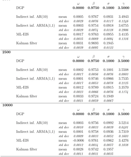
Evidence from simulated processes

values of the estimates computed later in this paper. The simulated series were estimated by indirect inference with an AR(10) and a ARMA(1,1) auxiliary model and by maximum EIS-computed likelihood. We also report the results of Kalman filter estimation, but only for the three parameters governing the dynamics of the latent variable, the only ones that would be estimated consistently by quasi maximum likelihood. The initial parameters of the four estimation methods were chosen to be equal to the simulation parameters plus a zero mean Gaussian error with standard deviation set at 0.05 for ω and β, at 0.01 for σ

and at 0.5 for γ. If any jittered starting value was beyond parameter constraints, a new sample of values was drawn. The parameters ω and β are estimated in a satisfactory way by all models even at the limited sample size of 1000 observations. Sample means and standard deviations are strictly comparable. Estimators seem to converge, in fact as the sample size increases, averages approach the simulated parameters and standard deviation become tighter. σ, the standard deviation of the innovations of the latent variable, seems more problematic to estimate. Indirect inference and ML-EIS seem to underestimate in a similar way, while the Kalman filter grossly overshoots (this last result is consistent with the Monte Carlo results in Bauwens and Galli (2009) for SCD models). Finally concerning

γ the shape parameter of the Weibull baseline, it seems that indirect inference with an ARMA(1,1) auxiliary model has a slight loss of efficiency compared with ML-EIS and AR(10)-based indirect inference.

4

Empirical analysis

4.1

The data

ranges were normalized to have a unit mean in order to speed up computation by reducing the search for the intercept in the conditional range function and to have more comparable estimates and forecasts. Out of the original 500 series, 22 of them were composed by less than 1000 observations and were discarded. This choice was somewhat arbitrary, but con-vergence issues for the numerical algorithms for very limited sample sizes required to set a threshold. Table 2 provides some descriptive statistics of the range series for the remaining 478 stocks. Not all series have a full 10 years length of 2517 observations, but the aver-age sample size after pruning our database of particularly short sets is quite close to the maximum value. It can be noted too that data have a rather low degree of overdispersion (computed as the ratio of sample mean and sample standard deviation), yet maxima tend to be several standard deviations away from the mean. Even visual inspection of some charts revealed that this could be due to an issue of outliers rather than to a particularly fat tail in the baseline distribution. Whether these outliers derive from quirks in recording or from exceptional conditions in the markets is difficult to tell. The use of an outlier detection and removal algorithm, like for instance the one deviced for durations by Chiang and Wang (2012), could be an interesting extension to this analysis and I leave it for further research. Average skewness and kurtosis indicate a strong departure from normality due to the presence of a heavy right tail. Statistics on autocorrelations are reported in the first column of the upper part of table 5 and show the presence of a marked degree of memory. These descriptive statistics are similar to the results obtained by Chou (2005).

4.2

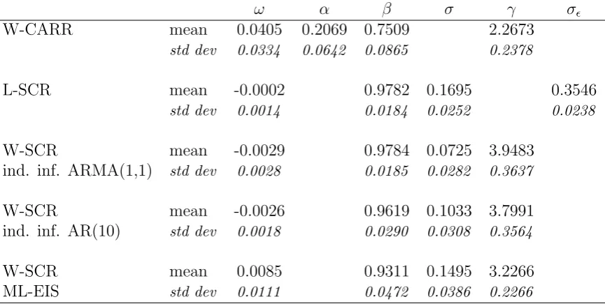
Estimation results

for conditional range. The first model was estimated by conditional maximum likelihood. In the second and the third model, likelihood was computed by respectively Kalman filter and EIS. The W-SCR model were also estimated by indirect inference with an AR(10) and an ARMA(1,1) as auxiliary models. Estimation times runned from less than a second for the CARR model to an average of half a minute for the L-SCR model and the W-SCR with an AR(10) auxiliary model and an average of 3-4 minutes for the W-SCR with ML-EIS and ARMA(1,1) indirect inference.

Table 3 reports sample means and standard deviations of the estimated parameters. All the estimators of the SCR model yield similar values for ω and forβ. The high level of persistence in the data is reflected by the average estimate ofβ, at a value close to one. In the CARR case a similar high persistence emerges from the sum of the estimated values of

α and β, which is close to one as well. Estimates for σ and γ seem to be sensitive to the method employed and seem to be negatively correlated. Even if the CARR model yields markedly lower estimates for γ than the SCR model, the parameter is always larger than 2 on average. This result is similar to the value obtained in Chou (2005) for the S&P500 index and suggest that an exponential distribution (that could be obtained by setting to one the γ parameter of the Weibull) would not be a suitable model for the baseline range.

4.3

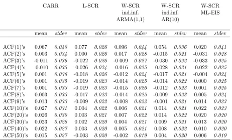
Analysis of residuals

For the SCR model, we can define the residual corresponding to the innovation ǫt as

ˆ

ǫt =Rt/e ˆ

ψt ₍₁₈₎

where ˆψt are the estimates of the latent variable provided either by the Kalman or the

where ˆΨt is recursively computed by replacing the values of the estimated parameters and

of Rt−₁ and Ψt−₁ in equation 3.

For each stock in the sample we computed the sample correlogram of ˆǫt and checked

if the strong autocorrelation present in the data was removed by the estimated dynamic part of the models we used. Results are detailed in table 4. Though none of the models seems to completely explain away the autocorrelation present in the data, residuals display a much limited serial dependence with respect to the samples used for estimation. The first autocorrelation is on average positive and quite high, followed by smaller negative values for the SCR models, while in the CARR case it drops close to zero after the first lag. At higher lags (after 10) SCR residuals’ autocorrelations tend to drop to small values while CARR’s ones show a tendency to increase.

4.4

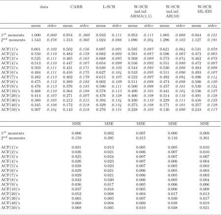
Fit of moments and autocorrelations

A comparison of the ability to fit the moments and autocorrelation structure of CARR and SCR models is presented in table 5. Moments and autocorrelations of the data were compared with implicit moments and autocorrelations computed by evaluating for each series formulae 4 to 7 and 10 to 12 with the values of estimated parameters.

Except for the W-SCR estimated with AR(10) indirect inference, all models seem to slightly underestimate the average of the data. The mean square errors of the first moments, computed by taking the average of the squares of differences between the empirical first moment and the implicit one computed on estimated parameters, show that the AR(10) W-SCR and the L-SCR seem to evaluate most precisely the mean of the process.

the data with a smaller square loss than L-SCD, which tends to overestimate the lower order autocorrelations and underestimate the higher order ones. CARR too has a higher value of MSE at all lags, as it systematically tends to underestimate the serial dependence in the data. It must be noted though that no model seems able to accont fully for the apparent long memory in the data and at high order of lags all autocorrelations seem to be underestimated.

4.5

Predictive accuracy

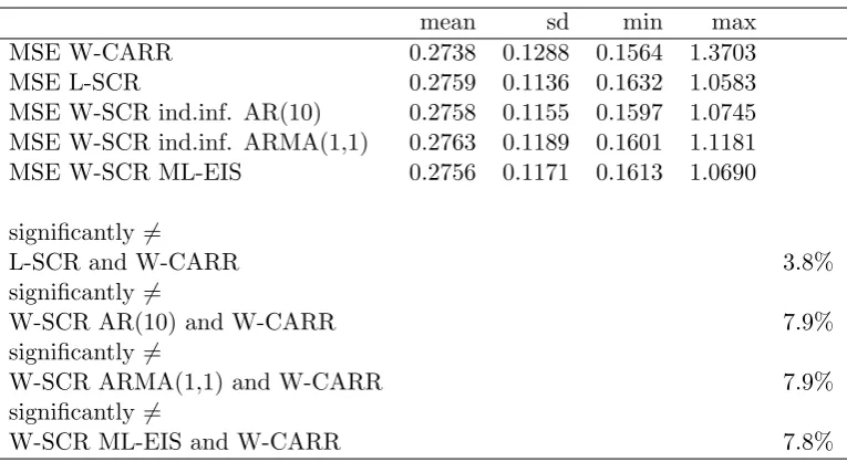
The predictive accuracy of the different models was compared by an insample one-step-ahead analysis. First the full sample was used to estimate the parameters of the models. Then we predicted every observation at time t = 2, ..., n using estimated parameters and observations at timet−1 = 1, ..., n−1. An outsample analysis was not performed because splitting the sample in two parts in an already quite short set of data woud either lead to more jittery parameter estimates or to too few forecasts.

The forecasting accuracy of each estimator for each series was measured by the mean square (prediction) error, that is the average of the squared difference between predicted and observed values. The significance of the difference between forecast errors of couples of estimators was verified by the Diebold and Mariano (2002) test with a bilateral alter-native and a quadratic loss function. Predictions are considered different if the Bonferroni corrected p-value is below 5%.

CARR expression for conditional range. The SCR could be augmented by including the past observed range as a further determinant of the dynamics of its latent component and it would be interesting to evaluate if its forecasting ability improves.

When the significance of pairs of forecasts is tested, it turns out that only about in one stock in fifteen the CARR and the W-SCR model forecast in a significantly different way. The proportion reduces of a half when the L-SCR is concerned. If finally we restrict our sample to significantly different forecasts only, we see that the gain of CARR in terms of MSE is slightly reduced in the case of the W-SCR while it remains substantially the same for the L-SCR.

We conclude by remarking that statistics on the comparisons between W-SCR and L-SCR, that are not reported in table 6, display a substantial similarity between the forecasts of the two models (for example, only less than the 1% of the forecasts can be considered different after testing).

5

Conclusion

The SCR is a simple model for the dynamics of financial range. Its estimation is feasible and can be achieved with several techiques, a few of them have been proposed here. In an empirical analysis on a large subset of the stocks composing S&P 500, SCR seemed to improve on the CARR model in reconstructing the autocorrelation structure of the data and was only slightly less efficient in forecasting.

References

Alizadeh, S., M. W. Brandt, and F. X. Diebold (2002): “Range-based estimation of stochastic volatility models,” The Journal of Finance, 57(3), 1047–1091.

Bauwens, L., and F. Galli (2009): “Efficient importance sampling for ML estimation of SCD models,”Computational Statistics and Data Analysis, 53(6), 1974–1992.

Bauwens, L., and N. Hautsch (2006): “Stochastic conditional intensity processes,”

Journal of Financial Econometrics, 4, 450–493.

Bauwens, L., and D. Veredas (2004): “The stochastic conditional duration model: a latent factor model for the analysis of financial durations,”Journal of Econometrics, 119(2), 381–412.

Bollerslev, T. (1986): “Generalized autoregressive conditional heteroskedasticity,”

Journal of Econometrics, 31, 307–327.

Brandt, M. W., and F. X. Diebold (2006): “A No-Arbitrage Approach to Range-Based Estimation of Return Covariances and Correlations,” Journal of Business, 79(1), 61–74.

Broto, C., and E. Ruiz (2004): “Estimation methods for stochastic volatility models: a survey,” Journal of Economic Surveys, 18(5), 613–649.

Chiang, M.-H., and L.-M. Wang (2012): “Additive Outlier Detection and Estimation for the Logarithmic Autoregressive Conditional Duration Model,” Communications in Statistics-Simulation and Computation, 41(3), 287–301.

Cox, D. R. (1981): “Statistical analysis of time series: Some recent developments [with discussion and reply],” Scandinavian Journal of Statistics, pp. 93–115.

Diebold, F. X., and R. S. Mariano(2002): “Comparing predictive accuracy,”Journal of Business & economic statistics, 20(1).

Engle, R. (1982): “Autoregressive conditional heteroskedasticity with estimates of the variance of United Kingdom inflation,”Econometrica, 50, 987–1007.

Engle, R., and J. R. Russell (1998): “Autoregressive conditional duration: a new approach for irregularly spaced transaction data,”Econometrica, 66, 1127–1162.

Gouri´eroux, C., and A. Monfort (1996): Simulation-based Econometric Methods. Oxford University Press.

Gourieroux, C., A. Monfort, and E. Renault(1993): “Indirect inference,”Journal of applied econometrics, 8(S1), S85–S118.

Knight, J., and C. Q. Ning (2008): “Estimation of the stochastic conditional duration model via alternative methods - ECF and GMM,”Econometrics Journal, 11(3), 593–616.

Liesenfeld, R., and J. F. Richard (2003): “Univariate and multivariate stochastic volatility models: estimation and diagnostics,” Journal of Empirical Finance, 10(4), 505–531.

Parkinson, M. (1980): “The extreme value method for estimating the variance of the rate of return,”Journal of Business, 53(1), 61.

Richard, J. F., and W. Zhang (2007): “Efficient high-dimensional importance sam-pling,”Journal of Econometrics, 141(2), 1385–1411.

Sanjeev Arulampalam, M., S. Maskell, N. Gordon, and T. Clapp (2002): “A tutorial on particle filters for online nonlinear/non-Gaussian Bayesian tracking,” Signal Processing, IEEE Transactions on, 50(2), 174–188.

Strickland, C., C. Forbes,and G. Martin(2006): “Bayesian analysis of the stochas-tic conditional duration model,” Computational Statistics and Data Analysis, 50(9), 2247–2267.

Taylor, S. J.(2007): “Modelling financial time series,” .

A

Appendix

A.1

Brief description of the EIS numerical integration method

An importance sampling estimate for the integral

G(y) =

Z

Λ

g(y, λ)p(λ)dλ, (19)

where g is an integrable function with respect to a density p(λ) with support Λ and the vectorydenotes an observed data vector (which in our context corresponds to the observed ranges), is provided by

¯

GS,m(y, a) =

1

S

S

X

i=1

g(y,˜λi)

p(˜λi)

m(˜λi, a)

, (20)

The aim of efficient importance sampling (EIS) is to minimize the MC variance of the estimator in (20) by selecting optimally the parameters a of the importance function density m given a functional form for m (here, the Gaussian density).

A convenient choice for the auxiliary samplerm(ψt, at) is a parametric extension of the

natural sampler q(ψt|ψt−1, θ2), in order to obtain a good approximation of the integrand

without too heavy a cost in terms of analytical complexity. Following Liesenfeld and Richard (2003), we use by the following specification:

m(ψt, at) =

q(ψt|ψt−₁, θ₂)ea1,tψt+a2,tψ

2

t

R

q(ψt|ψt−₁, θ₂)ea1,tψt+a2,tψ

2

tdψ_t

, (21)

where at = (a1,t a2,t). This specification is rather straightforward and has the advantage

that the auxiliary sampler m(ψt, at) remains Gaussian.

The parameters at can be chosen such that they minimize the sampling variance

ˆ

at(θ) = arg min at

S

X

j=1

{lnhf(Rt,ψ˜ (j) t |ψ˜

(j)

t−₁, Rt−₁, θ)χ( ˜ψ

(j) t ,ˆat+1)

i

−ct−ln(k( ˜ψ (j)

t , at))}2, (22)

wherectis constant that must be estimated along withat. If the auxiliary samplerm(ψt, at)

belongs to the exponential family of distributions, the problem becomes linear in at, and

this greatly improves the speed of the algorithm, as a least squares formula can be employed instead of an iterative routine. EIS-ML estimates are finally obtained by maximizing

˜

A.2

Brief description of the method of indirect inference

We can define the model which is object of indirect inference estimation (estimand model) in the following way:

M ={g(wt|wt

−₁

;θ)} (23)

where wt−₁

= wt−₁, w_t−₂, ... and w_t = (R_t, ψ_t). Its conditional probability distribution

MSCR_{, can be determined by the two expressions in equations 8 and 9. The parameters}

of interest in this case would be θ′

= (ω, β, σ, γ). Simulating from M is possible and the resulting values are denoted R_T = {Rt, t = 1, ..., T} for a given value of the parameter

vector θ and given initial conditions w0 = (R0, ψ0). The auxiliary criterion is QT(RT, β)

and its maximization will lead to an estimate of β

ˆ

βT = arg maxβ QT(RT, β). (24)

The key assumption is that the criterion converges to a deterministic limitQ∞(θ, β), which

is a function of the distribution MSCR_{, and therefore of θ and β. The value of β which}

maximizes this limit is called the binding function:

ˆ

βT = arg maxβ Q∞(θ, β). (25)

An estimation of the binding function can be achieved through simulation from the esti-mand model. If we denote by RT H(θ) ={Rt(θ), t = 1, ...T H} a simulated vector from M

given a parameter θ and initial conditionsw0 and replace with it the observed data in the

above equation, an estimator of the binding function is given by:

˜

and an indirect inference estimator of the estimand model parameters θ is given by

˜

θH

T = arg minθ{βˆT −β˜T H(θ)}

′ˆ

ΩT{βˆT −β˜T H(θ)}, (27)

where ˆΩT is a positive definite weighting matrix converging to a deterministic positive

definite matrix Ω.

1000

ω β σ γ

DGP 0.0000 0.9750 0.1000 3.5000

Indirect inf. AR(10) mean 0.0005 0.9767 0.0931 3.4943

std dev 0.0029 0.0076 0.0117 0.1246

Indirect inf. ARMA(1,1) mean 0.0003 0.9754 0.0918 3.6755

std dev 0.0029 0.0074 0.0128 0.2906

ML-EIS mean 0.0017 0.9763 0.0955 3.4135

std dev 0.0035 0.0089 0.0094 0.1316

Kalman filter mean 0.0031 0.9693 0.1945

std dev 0.0039 0.0095 0.0122

2500

ω β σ γ

DGP 0.0000 0.9750 0.1000 3.5000

Indirect inf. AR(10) mean 0.0002 0.9753 0.1001 3.5508

std dev 0.0017 0.0056 0.0076 0.0803

Indirect inf. ARMA(1,1) mean 0.0001 0.9746 0.0966 3.7535

std dev 0.0017 0.0053 0.0078 0.2125

ML-EIS mean 0.0012 0.9789 0.0915 3.3570

std dev 0.0023 0.0066 0.0076 0.1174

Kalman filter mean 0.0033 0.9724 0.1949

std dev 0.0021 0.0059 0.0067

10000

ω β σ γ

DGP 0.0000 0.9750 0.1000 3.5000

Indirect inf. AR(10) mean 0.0003 0.9756 0.0992 3.5214

std dev 0.0010 0.0033 0.0039 0.0401

Indirect inf. ARMA(1,1) mean 0.0001 0.9758 0.0936 3.7319

std dev 0.0009 0.0033 0.0052 0.1603

ML-EIS mean -0.0006 0.9761 0.0962 3.4276

std dev 0.0012 0.0034 0.0057 0.1038

Kalman filter mean 0.0028 0.9742 0.1957

std dev 0.0011 0.0031 0.0035

mean std deviation maximum minimum observations 2469.176 201.072 2517 1039

means 1 0 1 1

medians 0.808 0.056 0.888 0.571 std deviations 0.720 0.158 1.489 0.499 minima 0.177 0.046 0.275 <0.001 maxima 9.586 5.294 45.431 4.303 skewnesses 3.745 2.414 25.621 1.758 kurtoses 34.378 91.415 981.904 5.442

Table 2: Descriptive statistics of the 478 stocks used for the empirical analysis.

ω α β σ γ σǫ

W-CARR mean 0.0405 0.2069 0.7509 2.2673

std dev 0.0334 0.0642 0.0865 0.2378

L-SCR mean -0.0002 0.9782 0.1695 0.3546

std dev 0.0014 0.0184 0.0252 0.0238

W-SCR mean -0.0029 0.9784 0.0725 3.9483 ind. inf. ARMA(1,1) std dev 0.0028 0.0185 0.0282 0.3637

W-SCR mean -0.0026 0.9619 0.1033 3.7991 ind. inf. AR(10) std dev 0.0018 0.0290 0.0308 0.3564

W-SCR mean 0.0085 0.9311 0.1495 3.2266 ML-EIS std dev 0.0111 0.0472 0.0386 0.2266

CARR L-SCR W-SCR W-SCR W-SCR

ind.inf. ind.inf. ML-EIS

ARMA(1,1) AR(10)

mean stdev mean stdev mean stdev mean stdev mean stdev

ACF(1)’s 0.067 0.040 0.077 0.026 0.096 0.044 0.054 0.036 0.020 0.041

ACF(2)’s 0.003 0.034 0.000 0.026 0.017 0.028 -0.015 0.021 -0.031 0.028

ACF(3)’s -0.011 0.036 -0.022 0.026 -0.009 0.027 -0.030 0.022 -0.033 0.025

ACF(4)’s -0.010 0.035 -0.026 0.024 -0.016 0.025 -0.028 0.021 -0.022 0.025

ACF(5)’s 0.001 0.036 -0.018 0.026 -0.012 0.024 -0.017 0.021 -0.004 0.024

ACF(6)’s 0.001 0.035 -0.019 0.023 -0.014 0.025 -0.014 0.022 0.000 0.025

ACF(7)’s 0.001 0.033 -0.019 0.023 -0.015 0.026 -0.012 0.023 0.001 0.025

ACF(8)’s 0.003 0.033 -0.017 0.023 -0.014 0.025 -0.009 0.023 0.005 0.024

ACF(9)’s 0.013 0.033 -0.009 0.022 -0.008 0.022 -0.001 0.021 0.014 0.023

ACF(10)’s 0.027 0.031 0.004 0.022 0.006 0.021 0.014 0.021 0.022 0.023

ACF(20)’s 0.026 0.030 0.003 0.021 0.007 0.022 0.014 0.022 0.020 0.020

ACF(30)’s 0.023 0.028 0.002 0.020 0.004 0.021 0.009 0.021 0.013 0.020

ACF(40)’s 0.022 0.027 0.003 0.020 0.005 0.021 0.008 0.022 0.010 0.020

ACF(50)’s 0.015 0.027 -0.003 0.020 -0.002 0.019 0.004 0.020 0.006 0.019

data CARR L-SCR W-SCR W-SCR W-SCR ind.inf. ind.inf. ML-EIS ARMA(1,1) AR(10)

mean stdev mean stdev mean stdev mean stdev mean stdev mean stdev

1st_{moments 1.000 0.000 0.954 0..060 0.933 0.111 0.953 0.111 1.005 0.066 0.944 0.121} 2nd_{moments 1.543 0.278 1.313 0.360 1.024 0.086 1.090 0.204 1.296 0.103 1.127 0.191}

ACF(1)’s 0.601 0.102 0.502 0.156 0.697 0.091 0.595 0.087 0.621 0.064 0.531 0.059

ACF(2)’s 0.550 0.110 0.483 0.159 0.682 0.092 0.581 0.087 0.596 0.067 0.473 0.065

ACF(3)’s 0.525 0.111 0.465 0.163 0.668 0.095 0.569 0.089 0.573 0.074 0.462 0.072

ACF(4)’s 0.513 0.110 0.447 0.167 0.654 0.099 0.556 0.092 0.551 0.080 0.472 0.087

ACF(5)’s 0.503 0.111 0.431 0.171 0.640 0.102 0.544 0.093 0.530 0.086 0.484 0.098

ACF(6)’s 0.494 0.111 0.416 0.175 0.627 0.104 0.533 0.095 0.511 0.090 0.493 0.107

ACF(7)’s 0.482 0.113 0.402 0.179 0.615 0.107 0.522 0.097 0.492 0.094 0.496 0.114

ACF(8)’s 0.475 0.112 0.389 0.182 0.602 0.109 0.511 0.098 0.474 0.098 0.506 0.120

ACF(9)’s 0.476 0.113 0.376 0.185 0.590 0.111 0.500 0.099 0.457 0.101 0.530 0.124

ACF(10)’s 0.468 0.110 0.364 0.188 0.578 0.113 0.490 0.101 0.441 0.104 0.536 0.127

ACF(20)’s 0.414 0.107 0.271 0.207 0.476 0.128 0.400 0.108 0.314 0.116 0.491 0.128

ACF(30)’s 0.380 0.105 0.212 0.215 0.394 0.134 0.330 0.110 0.229 0.111 0.416 0.122

ACF(40)’s 0.345 0.108 0.172 0.218 0.329 0.134 0.273 0.108 0.171 0.101 0.357 0.129

ACF(50)’s 0.307 0.104 0.143 0.218 0.276 0.131 0.228 0.103 0.130 0.090 0.243 0.117

MSE MSE MSE MSE MSE

1st_{moments 0.006 0.002 0.007 0.000 0.009} 2nd_{moments 0.159 0.395 0.315 0.116 0.301}

ACF(1)’s 0.031 0.013 0.005 0.005 0.010 ACF(2)’s 0.026 0.021 0.006 0.007 0.010 ACF(3)’s 0.025 0.024 0.007 0.007 0.007 ACF(4)’s 0.026 0.023 0.007 0.006 0.004 ACF(5)’s 0.028 0.023 0.007 0.005 0.003 ACF(6)’s 0.029 0.021 0.006 0.005 0.003 ACF(7)’s 0.029 0.021 0.006 0.005 0.003 ACF(8)’s 0.032 0.020 0.006 0.005 0.004 ACF(9)’s 0.036 0.017 0.005 0.006 0.006 ACF(10)’s 0.037 0.016 0.005 0.006 0.008 ACF(20)’s 0.052 0.008 0.004 0.017 0.013 ACF(30)’s 0.065 0.005 0.007 0.030 0.017 ACF(40)’s 0.068 0.004 0.009 0.038 0.019 ACF(50)’s 0.068 0.005 0.010 0.038 0.021

mean sd min max

MSE W-CARR 0.2738 0.1288 0.1564 1.3703

MSE L-SCR 0.2759 0.1136 0.1632 1.0583

MSE W-SCR ind.inf. AR(10) 0.2758 0.1155 0.1597 1.0745

MSE W-SCR ind.inf. ARMA(1,1) 0.2763 0.1189 0.1601 1.1181

MSE W-SCR ML-EIS 0.2756 0.1171 0.1613 1.0690

significantly6=

L-SCR and W-CARR 3.8%

significantly6=

W-SCR AR(10) and W-CARR 7.9%

significantly6=

W-SCR ARMA(1,1) and W-CARR 7.9%

significantly6=

W-SCR ML-EIS and W-CARR 7.8%