S matrix for strings on η deformed AdS5 × S 5

JHEP04(2014)002

Received: January 30, 2014 Accepted: March 4, 2014 Published: April 1, 2014

S-matrix for strings on

η

-deformed

AdS

×

S

Gleb Arutyunov,a,1 Riccardo Borsatoa and Sergey Frolovb,c,1,2

a_{Institute for Theoretical Physics and Spinoza Institute, Utrecht University,}

Leuvenlaan 4, 3584 CE Utrecht, The Netherlands

b_{Institut f¨ur Mathematik und Institut f¨ur Physik, Humboldt-Universit¨at zu Berlin,}

IRIS Adlershof, Zum Großen Windkanal 6, 12489 Berlin, Germany

c_{Hamilton Mathematics Institute and School of Mathematics,}

Trinity College, Dublin 2, Ireland

E-mail: [email protected],[email protected],[email protected]

Abstract: We determine the bosonic part of the superstring sigma model Lagrangian

on η-deformed AdS5×S5, and use it to compute the perturbative world-sheet scattering matrix of bosonic particles of the model. We then compare it with the large string tension limit of the q-deformed S-matrix and find exact agreement.

Keywords: AdS-CFT Correspondence, Bosonic Strings, Exact S-Matrix, Integrable Field

Theories

ArXiv ePrint: 1312.3542

JHEP04(2014)002

1 Introduction 1

2 Superstrings on η-deformed AdS5×S5 3

3 Perturbative bosonic world-sheet S-matrix 6

3.1 Light-cone gauge and quartic Hamiltonian 6

3.2 Tree level bosonic S-matrix 9

3.3 Comparison with the q-deformed S-matrix 11

4 Conclusions 13

A The inverse operator and bosonic Lagrangian 14

B The psu(2|2)_q-invariant S-matrix 17

C Expansion of the q-deformed Gamma-function 19

1 Introduction

In recent years significant progress has been made towards understanding the excitation spectrum of strings moving in five-dimensional anti-de Sitter space-time and, accordingly, the spectrum of scaling dimensions of composite operators in planarN = 4 supersymmetric gauge theory. This progress became possible due to the fundamental insight that strings propagating in AdS space can be described by an integrable model. In certain aspects, however, the deep origin of this exact solvability has not yet been unraveled, mainly be-cause of tremendous complexity of the corresponding model. A related question concerns robustness of integrability in the context of the gauge-string correspondence [1], as well as the relationship between integrability and the amount of global (super)symmetries pre-served by the target space-time in which strings propagate. To shed further light on these important issues, one may attempt to search for new examples of integrable string back-grounds that can be solved by similar techniques. One such instance, where this program is largely promising to succeed, is to study various deformations of the string target space that preserve the integrability of the two-dimensional quantum field theory on the world sheet. Simultaneously, this should provide interesting new information about integrable string models and their dual gauge theories.

JHEP04(2014)002

giving a string theory on a TsT-transformed background [4,5]. Eventually all deformations of this class can be conveniently described in terms of the original string theory, where the deformations result into quasi-periodic but still integrable boundary conditions for the world-sheet fields.

The second class of deformations affects the AdS5 ×S5 model on a much more fun-damental level and is related to deformations of the underlying symmetry algebra. In the light-cone gauge this symmetry algebra constitutes two copies of the centrally extended Lie superalgebrapsu(2|2) with the same central extension for each copy. It appears that this centrally extended psu(2|2), or more precisely its universal enveloping algebra, admits a natural deformation psu_q(2|2) in the sense of quantum groups [6,7]. This algebraic struc-ture is the starting point for the construction of apsu_q(2|2)⊕psu_q(2|2)-invariant S-matrix, giving a quantum deformation of the AdS₅×S5 world-sheet S-matrix [6,8,9]. The defor-mation parameter q can be an arbitrary complex number, but in physical applications is typically taken to be either real or a root of unity.

Since these quantum group deformations modify the dispersion relation and the scat-tering matrix, to solve the corresponding model by means of the mirror Thermodynamic Bethe Ansatz (TBA), for a recent review see [10], one has to go through the entire procedure of first deriving the TBA equations for the ground state and then extending them to include excited states. While this program has been successfully carried out for deformations with

q being a root of unity [11, 12], the corresponding string background remains unknown. There is a conjecture that in the limit of infinite ’t Hooft coupling the q-deformed S-matrix tends to that of the Pohlmeyer-reduced version of the AdS5×S5 superstring [13,14]. It is not straightforward, however, to identify the S-matrix of the latter theory as one has to un-derstand whether the elementary excitations that scatter in that model are solitons or kinks. The case of real deformation parameter considered in this paper is not less compelling. Recently there was an interesting proposal on how to deform the sigma-model for strings on AdS5×S5 with a real deformation parameter η [15]. Deformations of this type con-stitute a general class of deformations governed by solutions of the classical Yang-Baxter equation [16,17]. This class is not solely restricted to the string model in question but can be applied to a large variety of two-dimensional integrable models based on (super)groups or their cosets [18]–[21].

The aim of the present work is to compute the 2 → 2 scattering matrix for the η -deformed model in the limit of large string tension g and to compare the corresponding result with the known q-deformed S-matrix found from quantum group symmetries, uni-tarity and crossing [6, 8]. In the context of the undeformed model a computation of this type has been carried out in [22].

JHEP04(2014)002

Let us summarize the results of this paper. Coming back to the bosonic action, we find that it corresponds to a string background which in addition to the metric also supports a non-vanishingB-field. The deformation breaks AdS₅×S5isometries down to U(1)3×U(1)3, where the first and second factors refer to the deformed AdS and five-sphere, respectively. Thus, only isometries corresponding to the Cartan elements of the isometry algebra of the AdS₅×S5 survive, very similar to the case of genericγ-deformations. As for the metric, its AdS part exhibits a singularity whose nature is currently unclear. Computed in a string frame the metric includes the contribution of a dilaton, and to extract the latter one needs to know the RR-fields which requires considering fermions.

With the bosonic action at hand it is straightforward to compute the corresponding tree-level S-matrix. We then show that it matches perfectly with the q-deformed S-matrix taken in the large tension limit and restricted to the scattering of bosons, provided we identify the deformation parameters as

q =e−ν/g, ν= 2η 1 +η2 .

This is the main result of our work which makes it quite credible that the η-deformed model indeed may enjoy hidden psu_q(2|2)⊕psu_q(2|2) symmetry for finite values of the coupling constantg. If true, this implies that despite the singular behaviour of the metric the quantum string sigma model would be well defined. In particular it would be possible to compute its exact spectrum by means of the mirror TBA.

The paper is organized as follows. In the next section we recall the general form of the action for the η-deformed model and use it to derive an explicit form of the Lagrangian for bosonic degrees of freedom. In section 3, upon fixing the uniform light-cone gauge, the corresponding Hamiltonian is derived up to quartic order in fields and further used to compute the tree-level S-matrix. This result is subsequently compared to the one arising from the q-deformed S-matrix (which includes the dressing phase) in the large g limit. We conclude by outlining interesting open problems. Finally some technical details on the derivation of the bosonic Lagrangian, the perturbative expansion of the q-deformed dressing phase and the form of the q-deformed S-matrix are collected in three appendices.

2 Superstrings on η-deformed AdS5×S5

According to [15], the action for superstrings on the deformed AdS5×S5 is

S = Z

dσdτL ,

where the Lagrangian density depending on a real deformation parameterη is given by1

L =−g 4(1 +η

2_{) γ}αβ ₋αβ str

˜

d(Aα) 1 1−ηRg◦d

(Aβ)

. (2.1)

1_{Note that ourη-dependent prefactor differs from the one in [15]. Our choice is necessary to match the}

JHEP04(2014)002

Here and in what follows we use the notations and conventions from [24], in particularτ σ = 1 andγαβ =hαβ√−hthat is the Weyl invariant combination of the world-sheet metrichαβ; the component γτ τ <0. The coupling constant g is the effective string tension. Further,

Aα = −g−1∂αg, where g ≡ g(τ, σ) is a coset representative from PSU(2,2|4)/SO(4,1)×

SO(5). To define the operators dand ˜dacting on the currents Aα, we need to recall that the Lie superalgebra G =psu(2,2|4) admits a_Z4-graded decomposition

G =G(0)⊕G(1)_⊕G(2)_⊕G(3)_.

Here G(0) coincides with so(4,1)×so(5). Denoting by Pi, i = 0,1,2,3, projections on the corresponding components of the graded decomposition above, operators dand ˜dare defined as

d= P1+ 2

1−η2P2−P3,

˜

d= −P1+ 2

1−η2P2+P3.

Finally, the action of the operatorRg onM ∈G is given by

Rg(M) =g−1R(gMg−1)g, (2.2)

where R is a linear operator onG satisfying the modified classical Yang-Baxter equation. In the following we define the action ofR on an arbitrary 8×8 matrix M as

R(M)_ij =−i ijMij, ij =   

 

1 if i < j

0 if i=j

−1 if i > j

, (2.3)

In the limit η → 0 one recovers from (2.1) the Lagrangian density of the AdS5×S5 superstring.

Our goal now is to obtain an explicit form for the corresponding bosonic action. With fermionic degrees of freedom switched off, formula (2.1) simplifies to

L =−g 2(1 +κ

2₎1_{2 γ}αβ₋αβ str

A(2)_α 1

1−_κRg◦P2 (Aβ)

, (2.4)

where we have introduced

κ= 2η

1−η2 ,

which as we see in a moment is a convenient deformation parameter.

To proceed, we need to choose a representative g of a bosonic coset SU(2,2|4)× SU(4)/SO(4,1)×SO(5) and invert the operator 1−ηRg◦d. A convenient choice of a coset

representative and the inverse of 1−ηRg◦dare discussed in appendix A. Making use of

the inverse operator, one can easily compute the corresponding bosonic Lagrangian. It is given by the sum of the AdS and sphere parts

JHEP04(2014)002

where we further split each part into the contribution of the metric and Wess-Zumino pieces. Accordingly, for the metric pieces we obtain

LG

a =−

g

2(1 +κ 2₎1

2 γαβ

−∂αt∂βt 1 +ρ

2

1−_κ2_ρ2 +

∂αρ∂βρ

(1 +ρ2_{) (1−κ}2_ρ2₎ +

∂αζ∂βζρ2

1 +_κ2_ρ4_sin2_ζ

+∂αψ1∂βψ1ρ 2_cos2_ζ

1 +κ2ρ4sin2ζ

+∂αψ2∂βψ2ρ2sin2ζ

, (2.6)

LG

s =−

g

2(1 +κ

2₎1_{2 γ}αβ∂αφ∂βφ 1−r2

1 +_κ2_r2 +

∂αr∂βr

(1−r2_{) (1 +}

κ2r2)

+ ∂αξ∂βξr 2

1 +_κ2_r4_sin2_ξ

+∂αφ1∂βφ1r 2_cos2_ξ

1 +_κ2_r4_sin2_ξ +∂αφ2∂βφ2r

2_sin2_{ξ, (2.7)}

while the Wess-Zumino partsL_aW Z and L_sW Z read

LW Z

a =

g

2κ(1 +κ 2₎1

2 αβ ρ 4_{sin 2ζ}

1 +_κ2_ρ4_sin2_ζ∂αψ1∂βζ , (2.8)

LW Z

s =−

g

2κ(1 +κ

2₎1₂ αβ r4sin 2ξ

1 +κ2r4sin2ξ∂αφ1∂βξ .

(2.9)

Here the coordinates t , ψ1, ψ2, ζ , ρ parametrize the deformed AdS space, while the co-ordinates φ , φ1, φ2, ξ , r parametrize the deformed five-sphere. Switching off the defor-mation, one finds that the AdS₅ coordinates are related to the embedding coordinatesZA, A= 0,1, . . . ,5 obeying the constraint ηABZAZB=−1 where ηAB = (−1,1,1,1,1,−1) as

Z1+iZ2 =ρcosζ eiψ1, Z3+iZ4 =ρsinζ eiψ2, Z0+iZ5 = q

1 +ρ2_eit_{, (2.10)}

while theS5coordinates are related to the embedding coordinatesYA, A= 1, . . . ,6 obeying Y_A2 = 1 as

Y1+iY2 =rcosξ eiφ1, Y3+iY4=rsinξ eiφ2, Y5+iY6 = p

1−r2_eiφ_{. (2.11)}

It is obvious that the deformed action is invariant under U(1)3×U(1)3 corresponding to the shifts of t,ψk, φ, φk. One also finds the ranges ofρ and r: 0 ≤ρ ≤ _κ1 and 0≤r ≤1.

The (string frame) metric of the deformed AdS is singular at ρ = 1/κ. Since we do not know the dilaton it is unclear if the Einstein frame metric exhibits the same singularity. The bosonic Wess-Zumino terms signify the presence of a non-trivial background B-field which is absent in the undeformed case.

In the next section we are going to impose the light-cone gauge, take the decompact-ification limit and compute the bosonic part of the four-particle world-sheet scattering matrix. To this end, we first expand the Lagrangian (2.5) up to quartic order inρ,r and their derivatives, and then make the shifts ofρandras described in appendixA, cf. (A.18). Since we are interested in the perturbative expansion in powers of fields aroundρ= 0, the final step consists in changing the spherical coordinates to (zi, yi)i=1,...,4 as

z1+iz2 1−1

4z2

=ρcosζeiψ1_, z3+iz4 1− 1

4z2

=ρsinζeiψ2_{, z}2_≡z2

i , (2.12)

y1+iy2

1 +1₄y2 =rcosξe

iφ1_, y3+iy4

1 +1₄y2 =rsinξe

JHEP04(2014)002

with further expanding the resulting action up to the quartic order in z and y fields. In this way we find the following quartic Lagrangian

La=−

g

2(1 +κ

2₎1_{2 γ}αβ_{−1 + (1 +}

κ2)z2+ 1 2(1 +κ

2₎2_(z2₎2_∂ αt∂βt

+

1 + (1−κ2)z

2

2

∂αzi∂βzi

+ 2gκ(1 +κ2)

1 2(z2

3 +z24)αβ∂αz1∂βz2,

Ls=−

g

2(1 +κ

2₎1_{2 γ}αβ _{1−(1 +}

κ2)y2+ 1 2(1 +κ

2₎2_(y2₎2_∂αφ∂ βφ

+

1−1 2(1−κ

2_)y2

∂αyi∂βyi

−2gκ(1 +κ2)

1 2(y2

3+y42)αβ∂αy1∂βy2.

(2.13)

We point out that the metric part of this Lagrangian has a manifest SO(4)×SO(4) sym-metry which is however broken by the Wess-Zumino terms.

3 Perturbative bosonic world-sheet S-matrix

3.1 Light-cone gauge and quartic Hamiltonian

To fix the light-cone gauge and compute the scattering matrix, it is advantageous to use the Hamiltonian formalism. For the reader’s convenience we start with a general discussion on how to construct the Hamiltonian for the world-sheet action of the form

S=−g 2

Z r

−r

dσdτγαβ∂αXM∂βXNGM N −αβ∂αXM∂βXNBM N

, (3.1)

where GM N and BM N are the background metric and B-field respectively. In the first order formalism we introduce conjugate momenta

pM = δS

δX˙M =−gγ 0β_∂

βXNGM N+gX

0_N

BM N. (3.2)

The action can be rewritten as

S = Z r

−r

dσdτ pMX˙M + γ01 γ00C1+

1 2gγ00C2

!

, (3.3)

whereC1, C2 are the Virasoro constraints. They are given by

C1 = pMX0M, (3.4)

C2 = GM NpMpN −2gpMX0QGM NBN Q+g2X0PX0QBM PBN QGM N +g2X0MX0NGM N.

The first Virasoro constraint has the same form as in the undeformed case. In particular, the solution for x0− in terms of pµ, xµ will still be the same. When expressed in terms of

the conjugate momenta, the second constraint gets an explicit dependence on the B-field. To impose light-cone gauge, one first introduces light-cone coordinates

JHEP04(2014)002

The second Virasoro constraint can be written as

C2=G−−p2−+ 2G+−p+p−+G++p2₊

+g2G++x0−2+ 2g2G+−x₊0 x0−+g2G−−x0₊2+Hx,

(3.6)

where

G−−=a2G−_φφ1−(a−1)2G−_tt1, G+−=aG_φφ−1−(a−1)G−_tt1, G++=G−_φφ1−G−_tt1,

G++= (a−1)2Gφφ−a2Gtt, G+−=−(a−1)Gφφ+aGtt, G−−=Gφφ−Gtt,

and Hx is the part that depends on the transverse fields only

H_x=Gµνpµpν +g2X0µX0νGµν−2gpµX0ρGµνBνρ+g2X0λX0ρBµλBνρGµν. (3.7)

Notice that the B-field is contained only in Hx, since in the action it does not couple to

the derivatives ofx±. We impose the uniform light-cone gauge

x+=τ, p+= 1. (3.8)

Solving C2 = 0 for p− gives the Hamiltonian

H=−p−(pµ, xµ, x0µ). (3.9)

Formally the solution for the Hamiltonian is still given by eq. (2.16) of the review [24], with the only difference that now the components of the metric are deformed and thatH_x has also theB-field contribution. Rescaling the fields with powers ofgand expanding in g

one can findHn, namely the part of the Hamiltonian that is of order nin the fields. Then

the action acquires the form

S = Z

dτdσ

pµx˙µ− H2− 1

gH4− · · ·

, (3.10)

where the quadratic Hamiltonian is given by

H2 = 1 2p

2 µ+

1 2(1 +κ

2_)x2 µ+

1 2(1 +κ

2_)x02

µ. (3.11)

The quartic Hamiltonian in a general a-gauge is

H4= 1 4

(2κ2z2−(1 +κ2)y2)p2z−(2κ2y2−(1 +κ2)z2)p2y

+1 +κ2 2z2−

1 +κ2

y2z02+1 +κ2

z2−2y2y02

−2_κ1 +_κ2 1 2

z₃2+z2₄ pz1z

0

2−pz2z

0

1

−y₃2+y₄2 py1y

0

2−py2y

0

1

+(2a−1) 8

(p2_y+p2_z)2−(1 +κ2)2(y2+z2)2

+ 2(1 +κ2)(p2y +p2z)(y

02_+z02_{) + (1 +}

κ2)2(y02+z02)2−4(1 +κ2)(x0−)2

.

(3.12)

Here we use the notation p2

z ≡p2zi, p

2

JHEP04(2014)002

To simplify the quartic piece, we can remove the terms of the form p2

zy2 and p2yz2 by

performing a canonical transformation generated by

V = (1 +κ 2₎

4 Z

dσpyyz2−pzzy2

, (3.13)

where the shorthand notation pyy ≡ pyiyi, pzz ≡ pzizi was used. After this is done the quartic Hamiltonian is

H₄ = (1 +κ 2₎

2 (z

2_z02_−y2_y02_{) +}(1 +κ2)2 2 (z

2_y02_−y2_z02_{) +}κ2 2 (z

2_p2

z−y2p2y)

−2_κ(1 +_κ2)12 h

z₃2+z2₄ pz1z

0

2−pz2z

0

1

−y₃2+y₄2 py1y

0

2−py2y

0

1 i

+(2a−1) 8

(p2_y+p2_z)2−(1 +_κ2)2(y2+z2)2 (3.14)

+2(1 +_κ2)(p2_y+p2_z)(y02+z02) + (1 +_κ2)2(y02+z02)2−4(1 +_κ2)(x0₋)2

.

We recall that in the undeformed case the corresponding theory is invariant with respect to the two copies of the centrally extended superalgebrapsu(2|2), each containing two su(2) subalgebras. To render invariance under su(2) subalgebras manifest, one can introduce two-index notation for the world-sheet fields. It is also convenient to adopt the same notation for the deformed case2

Z3 ˙4= 1₂(z3−iz4), Z3 ˙3= 1₂(z1−iz2),

Z4 ˙3=−1

2(z3+iz4), Z 4 ˙4₌ 1

2(z1+iz2),

(3.15)

Y1 ˙2= 1₂(y3−iy4), Y1 ˙1= 1₂(y1+iy2),

Y2 ˙1=−1

2(y3+iy4), Y 2 ˙2₌ 1

2(y1−iy2).

(3.16)

In terms of two-index fields the quartic Hamiltonian becomesH₄ =HG

4 +HW Z4 , whereHG4 is the contribution coming from the spacetime metric andHW Z

4 from the B-field

HG

4 = 2(1 +κ2)

Zαα˙Zαα˙Z_β0_β˙Z0β ˙ β_−Y

aa˙Yaa˙Y_b0_b˙Y0b ˙ b

+2(1 +_κ2)2Zαα˙Zαα˙Y_b0_b˙Y0b ˙ b_−Y

aa˙Yaa˙Z_β0_β˙Z0β ˙ β

+κ 2

2

Zαα˙Zαα˙P_ββ˙Pβ ˙ β_−Y

aa˙Yaa˙P_bb˙Pb ˙ b

+(2a−1) 8

₁

4(Paa˙P

aa˙ _+P

αα˙Pαα˙)2−4(1 +κ2)2(Yaa˙Yaa˙ +Zαα˙Zαα˙)2 (3.17)

+2(1+_κ2)(Paa˙Paa˙+Pαα˙Pαα˙)(Ya0a˙Y0aa˙+Zα0α˙Z0αα˙)+4(1+κ2)2(Ya0a˙Y0aa˙+Zα0α˙Z0αα˙)2

−4(1 +_κ2)(Paa˙Y0aa˙+Pαα˙Z0αα˙)2

,

HW Z₄ = 8iκ(1 +κ2)

1 2

Z3 ˙4Z4 ˙3(P_{3 ˙3}Z03 ˙3−P_{4 ˙4}Z04 ˙4) +Y1 ˙2Y2 ˙1(P_{1 ˙1}Y01 ˙1−P_{2 ˙2}Y02 ˙2).

2_{This parameterisation is different from the one used in [24] and the difference is the exchange of the}

definitions forY1 ˙1 _andY2 ˙2_{. This does not matter in the undeformed case but is needed here in order to}

JHEP04(2014)002

Note that we have used the Virasoro constraint C1 in order to express x0− in terms of

the two index fields. The gauge dependent terms multiplying (2a−1) are invariant under SO(8) as in the underformed case.

3.2 Tree level bosonic S-matrix

The computation of the tree level bosonic S-matrix follows the route reviewed in [24], and we also use the same notations. It is convenient to rewrite the tree-level S-matrix as a sum of two terms _T=_TG+_TW Z, coming from HG

4 and H4W Z respectevely. The reason is that TG preserves the so(4)⊕so(4) symmetry, while TW Z breaks it. To write the results we always assume that p > p0. Then, one finds that the action of _TG on the two-particle states is given by

TG |YacY˙ _b0_d˙i= "

1−2a

2 (pω

0₋

p0ω) + 1 2

(p−p0)2+ν2(ω−ω0)2

pω0_−p0_ω

#

|YacY˙ _b0_d˙i

+pp

0_+ν2_ωω0

pω0_−p0_ω

|Y_ad˙Yb0c˙i+|Ybc˙Y_a0_d˙i

,

TG |ZαγZ˙ _β0_δ˙i= "

1−2a

2 (pω

0₋

p0ω)− 1 2

(p−p0)2+ν2(ω−ω0)2

pω0_−p0_ω

#

|ZαγZ˙ _β0_δ˙i

−pp

0_+ν2_ωω0

pω0_−p0_ω

|Z_αδ˙Zβ0γ˙i+|Zβγ˙Z_α0_δ˙i

,

TG |Y_ab˙Z_α0_β˙i= "

1−2a

2 (pω

0₋

p0ω)− ω

2_−ω02

pω0_−p0_ω

#

|Y_ab˙Z_α0_β˙i,

TG |Z_αβ˙Y_a0_b˙i= "

1−2a

2 (pω

0_−p0_ω

) + ω 2_−ω02

pω0−p0ω #

|Z_αβ˙Y_a0˙_bi,

(3.18)

and the action of TW Z on the two-particle states is

TW Z |Yac˙Y_b0_d˙i=iν

ab|Ybc˙Y_a0_d˙i+c˙d˙|Yad˙Y

0

bc˙i

,

TW Z |Zαγ˙Z_β0_δ˙i=iν

αβ|Zβγ˙Z_α0_δ˙i+γ˙δ˙|Zαδ˙Z

0

βγ˙i

,

(3.19)

where on the r.h.s. we obviously do not sum over the repeated indices. In the formulae the frequencyω is related to the momentum pas

ω = (1 +κ2)

1 2

q

1 +p2₌ s

1 +p2

1−ν2, (3.20)

and we have introduced the parameter

ν = κ (1 +κ2)

1 2

= 2η

1 +η2, (3.21)

JHEP04(2014)002

The S-matrix _Scomputed in perturbation theory is related to the _T-matrix as

S=1+ i

gT. (3.22)

In the undeformed case, as a consequence of invariance of _S with respect to two copies of the centrally extended superalgebrapsu(2|2), the corresponding_T-matrix admits a factor-ization

TP

˙ P ,QQ˙

MM ,N˙ N˙ = (−1)

M˙(N+Q)_TP Q

M Nδ ˙ P ˙ Mδ

˙ Q ˙

N+ (−1)

Q(M˙+P˙)_δP Mδ

Q NT

˙ PQ˙

˙

MN˙ . (3.23)

Here M = (a, α) and M˙ = ( ˙a,α˙), and dotted and undotted indices are referred to two copies of psu(2|2), respectively, while M and _M˙ describe statistics of the corresponding indices, i.e. they are zero for bosonic (Latin) indices and equal to one for fermionic (Greek) ones. The factorT can be regarded as 16×16 matrix.

It is not difficult to see that the same type of factorization persists in the deformed case as well. Indeed, from the formulae (3.18) we extract the following elements for the T-matrix

T_abcd=A δ_acδ_bd+B δ_adδc_b+W abδdaδcb,

T_αβγδ =D δ_αγδ_βδ+E δδ_αδ_βγ+W αβδαδδ γ β,

Tcδ

aβ =G δacδδβ, T γd αb =L δ

γ αδbd,

(3.24)

where the coefficients are given by

A(p, p0) = 1−2a 4 (pω

0_−p0_{ω) +}1

4

(p−p0)2+ν2(ω−ω0)2

pω0_−p0_ω ,

B(p, p0) =−E(p, p0) = pp

0_+ν2_ωω0

pω0_−p0_ω ,

D(p, p0) = 1−2a 4 (pω

0_−p0_ω)−1

4

(p−p0)2+ν2(ω−ω0)2

pω0_−p0_ω ,

G(p, p0) =−L(p0, p) = 1−2a 4 (pω

0_−p0_ω)−1

4

ω2−ω02 pω0−p0ω, W(p, p0) =iν .

(3.25)

HereW corresponds to the contribution of the Wess-Zumino term and it does not actually depend on the particle momenta. All the four remaining coefficients T_abγδ,Tcd

αβ,T γd aβ,T

γd αb

vanish in the bosonic case but will be switched on once fermions are taken into account. The matrix T is recovered from its matrix elements as follows

T =T_{M N}P QE_PM ⊗E_QN =T_abcdE_ca⊗E_db+T_αβγδE_γα⊗Eβ_δ +T_aβcδE_ca⊗E_δβ+T_αbγdEα_γ ⊗E_db,

JHEP04(2014)002

explicit 16×16 matrix3

T ≡



                           

A1 0 0 0 | 0 0 0 0 | 0 0 0 0 | 0 0 0 0

0 A2 0 0 | A4 0 0 0 | 0 0 0 0 | 0 0 0 0 0 0 A3 0 | 0 0 0 0 | 0 0 0 0 | 0 0 0 0 0 0 0 A3 | 0 0 0 0 | 0 0 0 0 | 0 0 0 0

− − − − − − − − − − − − − − − − − − −

0 A5 0 0 | A2 0 0 0 | 0 0 0 0 | 0 0 0 0 0 0 0 0 | 0 A1 0 0 | 0 0 0 0 | 0 0 0 0 0 0 0 0 | 0 0 A3 0 | 0 0 0 0 | 0 0 0 0 0 0 0 0 | 0 0 0 A3 | 0 0 0 0 | 0 0 0 0

− − − − − − − − − − − − − − − − − − −

0 0 0 0 | 0 0 0 0 | A8 0 0 0 | 0 0 0 0 0 0 0 0 | 0 0 0 0 | 0 A8 0 0 | 0 0 0 0 0 0 0 0 | 0 0 0 0 | 0 0 A6 0 | 0 0 0 0 0 0 0 0 | 0 0 0 0 | 0 0 0 A7 | 0 0 A9 0

− − − − − − − − − − − − − − − − − − −

0 0 0 0 | 0 0 0 0 | 0 0 0 0 | A8 0 0 0 0 0 0 0 | 0 0 0 0 | 0 0 0 0 | 0 A8 0 0 0 0 0 0 | 0 0 0 0 | 0 0 0 A10 | 0 0 A7 0 0 0 0 0 | 0 0 0 0 | 0 0 0 0 | 0 0 0 A6



                            .

Here the non-trivial matrix elements ofT are given by

A1 =A+B, A2=A, A4 =B−W, A5=B+W, A6 =D+E, (3.26)

A₆ =D+E, A₇=D, A₈ =L, A₉=E−W =−A₅, A₁₀=E+W =−A₄.

We conclude this section by pointing out that the found matrixT satisfies the classical Yang-Baxter equation

[T12(p1, p2),T13(p1, p3) +T23(p2, p3)] + [T13(p1, p3),T23(p2, p3)] = 0 (3.27)

for any value of the deformation parameter ν.

3.3 Comparison with the q-deformed S-matrix

In this subsection we show that the perturbative bosonic world-sheet S-matrix coincides with the first nontrivial term in the largegexpansion of the q-deformed AdS5×S5S-matrix, in other words with the corresponding classicalr-matrix.4

Let us recall that up to an overall factor the q-deformed AdS₅×S5 S-matrix is given by a tensor product of two copies of thepsu(2|2)q-invariant S-matrix [6] which is reviewed in

appendix B. Including the overall factorSsu(2) which is the scattering matrix in the su(2) sector, the complete S-matrix can be written in the form [8]

S=Ssu(2)S⊗ˆS , Ssu(2)=

eia(p2E1−p1E2) σ2

12

x+₁ +ξ x−₁ +ξ

x−₂ +ξ x+₂ +ξ ·

x−₁ −x+₂ x+₁ −x−₂

1− 1

x−₁x+₂

1− 1 x+₁x−₂

, (3.28)

whereS is thepsu(2|2)_q-invariant S-matrix (B.3), ˆ⊗stands for the graded tensor product,

a is the parameter of the light-cone gauge (3.5), σ is the dressing factor, and E is the

3_{See appendix 8.5 of [25] for the corresponding matrix in the undeformed case.}

4_{The difference with the expansion performed in [13] is that we include the dressing factor in the definition}

JHEP04(2014)002

q-deformed dispersion relation (B.9) whose large g expansion starts withω. The dressing factor can be found by solving the corresponding crossing equation, and it is given by [8]

σ12=eiθ12, θ12=χ(x+1, x+2) +χ(x

−

1, x

−

2)−χ(x+1, x

−

2)−χ(x

−

1, x+2), (3.29)

where

χ(x1, x2) =i I _dz

2πi

1

z−x1 I _dz0

2πi

1

z0_−x

2 log

Γ_q2

1 +ig₂(u(z)−u(z0))

Γ_q2

1−ig₂(u(z)−u(z0))

. (3.30)

Here Γ_q(x) is the q-deformed Gamma function which for complex q admits an integral representation (C.1) [8].

To develop the large g expansion of the q-deformed AdS₅×S5 S-matrix, one has to assume thatq =e−υ/g _{whereυis a deformation parameter which is kept fixed in the limit} g → ∞, and should be related to ν. Then, due to the factorisation of the perturbative bosonic world-sheet S-matrix and the q-deformed AdS₅ ×S5 S-matrix, it is sufficient to compare theT-matrix (3.24) with theT-matrix appearing in the expansion of the “square root” ofS

S_su1/₍₂₎2 1gS =1+ i

gT, (3.31)

where 1_g is the graded identity which is introduced so that the expansion starts with 1. The only term which is not straightforward to expand is the S_su(2) scalar factor because it contains the dressing phase θ12. The scalar factor obviously can contribute only to the part of the T-matrix proportional to the identity matrix. Since in the expansion of the psu(2|2)q-invariant S-matrix (B.3), 1gS =1+ _gir, the element r1111 is equal to 0 (because a1 = 1) it is convenient to subtract T11111 = A11 from the T-matrix and compare the resulting matrix with the classicalr-matrix. One should obviously remove the off-diagonal terms from the classical r-matrix which appear due to the presence of fermions in the full superstring action (2.1). With this done, one finds that they are equal to each other provided υ = ν, and therefore q = e−ν/g is real. Thus, to show that T = T one should demonstrate that A1 is equal to the 1/g term in the expansion of S_su1/₍₂₎2 . To this end one should find the largegexpansion of the dressing phaseθ12which is done by first expanding the ratio of Γ_q2-functions in (3.30) with u(z) and u(z0) being kept fixed. This is done in appendix C, see (C.9). Next, one combines it with the expansion of the 1

z−x±₁ 1 z0_−x±

2

terms

which appear in the integrand of (3.29). As a result one finds that the dressing phase is of order 1/gjust as it was in the undeformed case [26]. We have not tried to compute the resulting double integrals analytically but we have checked numerically that the element A1is indeed equal to the 1/gterm in the expansion ofS_su1/₍₂₎2 if the deformation parameterν

satisfiesν <1/√2. At ν= 1/√2 the integral representation for the dressing factor breaks down but it is unclear to us if it is a signal of a genuine problem with the q-deformed S-matrix. In fact it is not difficult to extract from A₁ the leading term in the large g

expansion of the dressing phase which appears to be very simple

θ12=

ν2(ω1−ω2) +p22(ω1−1)−p21(ω2−1) 2g(p1+p2)

JHEP04(2014)002

It would be curious to derive this expression from the double integral representation. Note that doing this double integral one also could get the full AFS order of the phase.

4 Conclusions

In this work we successfully matched in the large tension limit the tree-level bosonic S-matrix arising from the sigma-model on the deformed AdS5 × S5 space with the q-deformed S-matrix obtained from symmetries. There are many other important issues to be addressed.

We identified NSNS background fields in the string frame. More studies are needed however to extract RR fields since the latter couple directly to fermionic degrees of freedom. Rather intricate field redefinitions should be performed to bring the deformed action to the standard one for Type IIB superstring in an arbitrary supergravity background, thus allowing the identification of the full bosonic background. It might be easier in fact just to use the NSNS background fields and the type IIB supergravity equations of motion to find the full supergravity background [23].

Next, the matching of S-matrices, successful at tree level, can be further extended by computing admittedly more complicated loop corrections to the tree-level scattering matrix of the light-cone sigma-model; this also requires taking fermions into account. It is natural to expect that the deformation parameter ν undergoes a non-trivial renormalization to fit the parameterq entering the exact, i.e. all-loop, q-deformed S-matrix.

We also showed that in the large tension limit the conjectured dispersion relation (B.9) turns into the perturbative one (3.20). It would be interesting to find an η-deformed giant magnon solution [27] which would provide additional evidence in favour of (B.9). In the case of the finite angular momentum the corresponding solution would also provide important information about the structure of the finite size corrections [28] in theη-deformed theory. It is also interesting to find explicit spinning string solutions of theη-deformed bosonic sigma-model. Due to the singularity of the η-deformed AdS a particularly interesting solution to analyse would be the GKP string and its generalisation [29, 30]. Then, in the case of AdS, substituting the spinning Ansatz in the sigma-model equations of motion leads to the emergence [31] of the Neumann model, a famous finite-dimensional integrable system. One may hope that studies of the η-deformed sigma-model in this context may reveal new integrable finite-dimensional systems which can be described as deformations of the Neumann model. Furthermore, known finite-gap integration techniques can be applied to obtain a wider class of solutions that generalize the solutions of the Neumann system. Normally they are described by a certain algebraic curve which is supposed to emerge from the Bethe Ansatz based on the exact q-deformed S-matrix in the semi-classical limit. This would serve as another non-trivial check that the two models, one based on the explicitly known deformed action and the other based on the exact quantum group symmetry, have a good chance to describe the same physics.

JHEP04(2014)002

With the knowledge of a complete supergravity background and its symmetries for the deformed case, one can approach perhaps the most interesting question about the dual gauge theory. Since the deformation affects the isometries of the AdS space, the theory will be neither conformal nor Lorentz invariant. Since there is a B-field on the string theory side, one may expect that this theory is a non-commutative deformation of N = 4 super Yang-Mills in the sense of the Moyal star product with a hidden quantum group symmetry which would include the two copies of the psu_q(2|2) algebra. It would be fascinating to construct such a theory explicitly.

Acknowledgments

We thank Marius de Leeuw, Stijn van Tongeren and Benoit Vicedo for useful discussions. G.A. and R.B. acknowledge support by the Netherlands Organization for Scientific Re-search (NWO) under the VICI grant 680-47-602. The work by G.A. and R.B. is also a part of the ERC Advanced grant research programme No. 246974, “Supersymmetry: a window to non-perturbative physics” and of the D-ITP consortium, a program of the NWO that is funded by the Dutch Ministry of Education, Culture and Science (OCW). S.F. is supported by a DFG grant in the framework of the SFB 647 “Raum - Zeit - Materie. Analytische und Geometrische Strukturen” and by the Science Foundation Ireland under Grant 09/RFP/PHY2142.

A The inverse operator and bosonic Lagrangian

To find the bosonic part of the deformed Lagrangian one needs to choose a coset represen-tativeg, and invert the operator 1−ηRg◦d. We find useful the following parametrisation

of a bosonic coset element

gb= _g

a 0

0 gs

, ga= Λ(ψk) Ξ(ζ)ˇgρ(ρ), gs= Λ(φk) Ξ(ξ)ˇgr(r). (A.1)

Here the matrix functions Λ, Ξ and ˇg are defined as

Λ(ϕk) = exp 3 X

k=1 i

2ϕkhk !

, Ξ(ϕ) = 

    

cosϕ₂ sinϕ₂ 0 0 −sinϕ₂ cosϕ₂ 0 0

0 0 cosϕ₂ −sinϕ₂ 0 0 sinϕ₂ cosϕ₂



    

, (A.2)

ˇ gρ(ρ) =



    

ρ+ 0 0 ρ−

0 ρ+ −ρ− 0

0 −ρ− ρ+ 0 ρ− 0 0 ρ+



    

, ρ±=

q p

ρ2_{+ 1±1}

√

2 , (A.3)

ˇ gr(r) =



    

r+ 0 0 i r−

0 r+ −i r− 0

0 −i r− r+ 0 i r− 0 0 r+



    

, r±=

q

1±√1−r2

√

JHEP04(2014)002

where the diagonal matrices hi are given by

h1 = diag(−1,1,−1,1), h2= diag(−1,1,1,−1), h3 = diag(1,1,−1,−1). (A.5)

In the undeformed case the AdS5 coordinates t ≡ ψ3, ψ1, ψ2, ζ , ρ are related to the embedding coordinatesZA, A= 0,1, . . . ,5 obeying the constraint ηABZAZB =−1 where ηAB _{= (−1,1,1,1,1,−1) as follows}

Z1+iZ2 =ρcosζ eiψ1, Z3+iZ4 =ρsinζ eiψ2, Z0+iZ5 = q

1 +ρ2_eit_{, (A.6)}

while the S₅ coordinates φ ≡ φ3, φ1, φ2, ξ , r are related to the embedding coordinates YA_{, A= 1, . . . ,6 obeying Y}2

A= 1 as

Y1+iY2 =rcosξ eiφ1, Y3+iY4=rsinξ eiφ2, Y5+iY6 = p

1−r2_eiφ_{. (A.7)}

An important property of the coset representative (A.1) is that the Rg operator is

inde-pendent of the angles ψk andφk:

Rgb(M) =Rˇg(M), ˇg=

_ˇ

ga 0

0 ˇgs

, ˇga= Ξ(ζ)ˇgρ(ρ), ˇgs= Ξ(ξ)ˇgr(r). (A.8)

To compute the Lagrangian one needs to know the action of the operator 1/(1−ηRg◦d)

on the projection M(2) and Modd of an su(2|2) element M. This action on odd elements appears to be ˇg-independent

1 1−ηRˇg◦d

(Modd) = 1

+ηR◦d

1−η2 (Modd). (A.9)

This action onM(2) factorizes into a sum of actions onMa and Ms whereMa is the upper

left 4×4 block ofM(2), andMs is the lower right 4×4 block ofM(2). One can check that

the inverse operator is given by

1 1−ηRˇg◦d

(Ma) =

1+η 3_fa

31+η4f42a +η5ha53 (1−caη2)(1−daη2)

+ ηRˇg◦d+η 2_R

ˇ

g◦d◦Rˇg◦d

1−caη2

Ma,(A.10)

1 1−ηRˇg◦d

(Ms) =

1+η 3_fs

31+η4f42s +η5hs53 (1−csη2)(1−dsη2)

+ ηRˇg◦d+η 2_R

ˇ

g◦d◦Rˇg◦d

1−csη2

Ms

.(A.11)

Here

ca=

4ρ2

(1−η2₎2, da = −

4ρ4sin2ζ

(1−η2₎2 , cs=− 4r2

(1−η2₎2, ds=−

4r4sin2ξ

(1−η2₎2, (A.12)

f_k,ka −2(Ma) =

Rˇg◦d

k

−ca Rˇg◦d

k−2

(Ma), (A.13)

f_k,ks −2(Ms) =

Rˇg◦d

k

−cs Rˇg◦d

k−2

(Ms), (A.14)

da and ds appear in the identities

JHEP04(2014)002

and ha

53 and hs53 appear in

ha₅₃=f₅₃a −daf31a , hs53=f53s −dsf31s . (A.16)

The bosonic Lagrangian can then be easily computed and is given by (2.5)–(2.9). To find the quartic Lagrangian used for computing the bosonic part of the four-particle world-sheet scattering matrix, we first expand the Lagrangian (2.5) up to quartic order in ρ, r

and their derivatives

La=−

g

2(1 +κ 2₎1₂

γαβh−∂αt∂βt(1 + (1 +κ2)ρ2(1 +κ2ρ2)) +∂αρ∂βρ(1 + (κ2−1)ρ2)

+∂αψ1∂βψ1ρ2cos2ζ+∂αψ2∂βψ2ρ2sin2ζ+∂αζ∂βζρ2 i

−_καβρ4sin 2ζ∂αψ1∂βζ

,

(A.17)

Ls=−

g

2(1 +κ 2₎1

2

γαβh∂αφ∂βφ(1−(1 +κ2)r2(1−κ2r2)) +∂αr∂βr(1 + (1−κ2)r2)

+∂αφ1∂βφ1r2cos2ξ+∂αφ2∂βφ2r2sin2ξ+∂αξ∂βξr2 i

+_καβr4sin 2ξ∂αφ1∂βξ

.

Further, we make a shift

ρ→ρ−κ

2

4 ρ

3_{, r→r+} κ2 4 r

3 _(A.18)

so that the quartic action acquires the form

La = −

g

2(1 +κ

2₎1_2γαβh_{−∂αt∂βt1 + (1 +}

κ2)ρ2+1₂κ2(1 +κ2)ρ4

+

+∂αρ∂βρ1−ρ2−κ2 2 ρ

4_+ρ2₋κ2 2 ρ

4_∂αψ

1∂βψ1cos2ζ+∂αψ2∂βψ2sin2ζ+∂αζ∂βζ i

+g

2κ(1 +κ

2₎1₂αβ_ρ4_{sin 2ζ∂}

αψ1∂βζ , (A.19)

Ls = −

g

2(1 +κ

2₎1_2γαβh_∂ αφ∂βφ

1−(1 +_κ2)r2+₂1_κ2(1 +_κ2)r4+

+∂αr∂βr

1 +r2+κ2 2 r

4_+r2₊κ2 2 r

4_∂

αφ1∂βφ1cos2ξ+∂αφ2∂βφ2sin2ξ+∂αξ∂βξ i

−g

2κ(1 +κ 2₎1

2αβr4sin 2ξ∂_αφ₁∂_βξ . (A.20)

Changing the spherical coordinates to (zi, yi), see (2.12), and expanding the resulting action

up to the quartic order inzand y fields we get the quartic Lagrangian (2.13). Notice that the shifts of ρ and r in (A.18) were chosen so that the deformed metric expanded up to quadratic order in the fields would be diagonal.

It is also possible to choose a coset representative precisely in the same way as is done in the undeformed case, see [24] for details. Accordingly, for the metric pieces we obtain

LG

a = −

g

2(1 +κ

2₎1_2γαβh_−G

tt∂αt∂βt+Gzz∂αzi∂βzi+G(1)a zi∂αzizj∂βzj+

+G(2)a (z3∂αz4−z4∂αz3)(z3∂βz4−z4∂βz3) i

, (A.21)

LG

s = −

g

2(1 +κ

2₎1_2γαβh

Gφφ∂αφ∂βφ+Gyy∂αyi∂βyi+G (1)

s yi∂αyiyj∂βyj+

+G(2)s (y3∂αy4−y4∂αy3)(y3∂βy4−y4∂βy3) i

JHEP04(2014)002

Here the coordinateszi,i= 1, . . . ,4, andtparametrize the deformed AdS space, while the

coordinates yi, i = 1, . . . ,4, and the angle φ parametrize the deformed five-sphere. The components of the deformed AdS metric in (A.21) are5

Gtt =

(1 +z2/4)2

(1−z2_/4)2_−κ2_z2, Gzz =

(1−z2/4)2 (1−z2_/4)4_+κ2_z2_(z2

3+z42) ,

G(1)a =κ2GttGzz z

2

3+z42+ (1−z2/4)2 (1−z2_/4)2_{(1 +z}2_/4)2 , G

(2)

a =κ2Gzz z

2

(1−z2_/4)4.

(A.23)

For the sphere part the corresponding expressions read

Gφφ =

(1−y2/4)2

(1 +y2_/4)2_+κ2_y2 , Gyy =

(1 +y2/4)2 (1 +y2_/4)4_+κ2_y2_(y2

3+y42) ,

G(1)s =κ2GφφGyy

y2₃+y₄2−(1 +y2/4)2 (1−y2_/4)2_{(1 +y}2_/4)2 , G

(2)

s =κ2Gyy y

2

(1 +y2_/4)4.

(A.24)

Obviously, in the limit _κ → 0 the components G(ai) and G(si) vanish, and one obtains the

metric of the AdS₅ ×S5, cf. fomulae (1.145) and (1.146) in [24]. Finally, for the Wess-Zumino terms the results (up to total derivative terms which do not contribute to the action) are

LW Z

a = 2gκ(1 +κ2)

1

2 αβ (z 2

3+z42)∂αz1∂βz2 (1−z2_/4)4_+κ2_z2_(z2

3+z42)

LW Z

s =−2gκ(1 +κ2)

1 2 αβ

(y2

3+y42)∂αy1∂βy2 (1 +y2_/4)4₊

κ2y2(y32+y42) .

(A.25)

To complete our discussion of the bosonic Lagrangian of the deformed theory, let us note that in the undeformed case the action is invariant with respect to two copies of SO(4) acting linearly onzi and yi respectively. As is seen from the expressions above, this symmetry is broken down to four copies of SO(2) ∼ U(1). Thus, together with the two U(1) isometries acting ontand φthe deformed action is invariant under U(1)3×U(1)3.

B The psu(2|2)q-invariant S-matrix

The S-matrix compatible with psu(2|2)q symmetry [6] has been studied in detail in the

recent papers [8, 11, 12, 14]. To make the present paper self-contained, in this appendix we recall its explicit form following the same notation as in [11].

Let Eij ≡Eij stand for the standard matrix unities, i, j= 1, . . . ,4. We introduce the

following definition

Ekilj = (−1)(l)(k)Eki⊗Elj, (B.1)

where (i) denotes the parity of the index, equal to 0 for i = 1,2 (bosons) and to 1 for

i= 3,4 (fermions). The matricesEkilj are convenient to write down invariants with respect

5_{Note that the coordinatesy}

JHEP04(2014)002

to the action of copies of su_q(2)⊂psu_q(2|2). If we introduce

Λ1 = E1111+ q

2E1122+ 1 2(2−q

2_)E 1221+

1

2E2112+

q

2E2211+E2222,

Λ₂ = 1

2E1122−

q

2E1221− 1

2qE2112+

1 2E2211,

Λ3 = E3333+ q

2E3344+ 1 2(2−q

2_)E 3443+

1

2E4334+

q

2E4433+E4444,

Λ4 = 1

2E3344−

q

2E3443− 1

2qE4334+

1 2E4433,

Λ₅ = E1133+E1144+E2233+E2244, (B.2)

Λ₆ = E3311+E3322+E4411+E4422,

Λ7 = E1324−qE1423− 1

qE2314+E2413,

Λ₈ = E3142−qE3214− 1

qE4132+E4231,

Λ₉ = E1331+E1441+E2332+E2442,

Λ₁₀ = E3113+E3223+E4114+E4224,

the S-matrix of the q-deformed model is given by

S12(p1, p2) = 10 X

k=1

ak(p1, p2)Λk, (B.3)

where the coefficients are

a1 = 1,

a2 = −q+ 2

q

x−₁(1−x−₂x₁+)(x+₁ −x+₂)

x+₁(1−x−₁x₂−)(x−₁ −x+₂)

a3 = U2V2 U1V1

x+₁ −x−₂ x−₁ −x+₂

a4 = −q U2V2 U1V1

x+₁ −x−₂ x−₁ −x+₂ +

2

q U2V2 U1V1

x−₂(x+₁ −x₂+)(1−x−₁x+₂)

x+₂(x−₁ −x₂+)(1−x−₁x−₂)

a5 =

x+₁ −x+₂

√

q U1V1(x−1 −x+2)

a6 =

√

q U2V2(x−1 −x

−

2)

x−₁ −x+₂ (B.4)

a7 = ig

2

(x+₁ −x−₁)(x+₁ −x+₂)(x+₂ −x−₂) √

q U1V1(x−1 −x+2)(1−x

−

1x

−

2)γ1γ2

a8 = 2i

g

U2V2x−1x

−

2(x + 1 −x

+ 2)γ1γ2 q32x+

1x + 2(x

−

1 −x + 2)(x

−

1x

−

2 −1)

a9 =

(x−₁ −x+₁)γ2 (x−₁ −x+₂)γ1

a10 =

U2V2(x−2 −x+2)γ1 U1V1(x−1 −x

+ 2)γ2

JHEP04(2014)002

Here the basic variables x± parametrizing a fundamental representation of the centrally extended superalgebra psu_q(2|2) satisfy the following constraint [6]

1

q

x++ 1

x+

−q

x−+ 1

x−

=

q−1

q ξ+

1

ξ

, (B.5)

where the parameter ξ is related the coupling constant g as

ξ=−i 2

g(q−q−1) q

1−g₄2(q−q−1₎2

. (B.6)

The (squares of) central charges are given by

U_i2 = 1

q

x+_i +ξ x−_i +ξ =e

ipi_{, V}2

i =q x+_i x−_i

x−_i +ξ

x+_i +ξ, (B.7)

and the parameters γi are

γi=q 1 4

s ig

2(x

−

i −x +

i )UiVi. (B.8)

The q-deformed dispersion relationE takes the form

1−g

2

4(q−q

−1₎2 !

qE/2−q−E/2 q−1/q

!2

−g2sin2 p 2 =

q1/2−q−1/2 q−1/q

!2

. (B.9)

Finally, we point out that in the q-deformed dressing phase the variableu appears which is given by

u(x) = 1

υlog "

−x+

1 x +ξ+

1 ξ ξ−1

ξ #

. (B.10)

C Expansion of the q-deformed Gamma-function

We take q =eiυ/g, keep x fixed and send g → ∞. We are interested in the leading term only. At the end we analytically continue to imaginaryυ. We have [8]

logΓq2(1+gx) Γ_q2(1−gx)

=−iυx+ Z ∞

0 dt

t

2 e−υxt−eυxt

eυtg _−1(eπt₋₁₎

−gπ e

−υxt_−eυxt

υ(eπt₋₁₎2 −

υ e−υxt−eυxt

gπeυtg ₋₁

2

+gπ e

−υxt_−eυxt

υ(eπt₋₁₎2 −

υ e−υxt−eυxt

gπeυtg ₋₁

2 + 2gxeυtg

eπt₋₁ +

2gxet π+υg

eπt₋₁ +

e−υxt−eυxt

eυtg ₋₁ +e

−υxt_−eυxt

eπt₋₁ !

.

(C.1)

We understand integrals of the formR∞

0 dtF(t) as in [33]

Z ∞

0

dt F(t)≡

Z

C0 dt

JHEP04(2014)002

C0

t

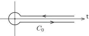
Figure 1. The integration contourC0 in the integral

R

C0 dt

2πiF(t) ln(−t).

where the integration contourC0 goes from +∞+i0 above the real axis, then around zero, and finally below the real axis to +∞ −i0, see figure1. Then the terms on the second line of (C.1) can be easily computed by using the functions introduced in [34]6

F2(z, a) ≡ Z ∞

0 dt

t

ezat

(eat₋₁₎2 = 13 12 +

z2 2 −

3z

2 −γ

z2 2 −z+

15 12

!

+ (z−1)logΓ(2−z)

+ψ(−2)(2−z)−log(A)−1

2log(2π)−

z2

2 −z+ 15 12

! loga ,

F1(z, a) ≡ Z ∞

0 dt

t ezat

eat₋₁ =F2(z+ 1, a)−F2(z, a)

=−γ

z−1 2

+ logΓ(1−z)−zloga+1 2log

_a

2π

, (C.3)

F0(z) ≡ Z ∞

0 dt

t e zt_=F

1(z+ 1,1)−F1(z,1) =−γ−log(−z),

whereψ(−2)(z) is given by

ψ(−2)(z) = Z z

0

dtlogΓ (t), (C.4)

and A is Glaisher’s constant which satisfies log(A) = 1/12−ζ0(−1) and ζ is the Riemann zeta function.

Thus, the terms on the second line of (C.1) are equal to

i2 = gπ υ F2 −υx

π , π

−F2 _υx

π , π + υ gπ F2

−gx,υ g

−F2

gx,υ g

+2gxF1 _υ

πg, π

+ 2gxF1

1− υ

πg, π

+F1

−gx,υ g

−F1

gx,υ g

+F1

−υx

π , π

−F1 _υx

π , π

. (C.5)

The integral on the first line of (C.1) is convergent at t = 0, and one can expand the integrand in powers of 1/g. One gets for the leading term

i1 =g Z ∞

0 dt

t

_{2 sinh(υxt)}

πυt2 +

4 sinh(υxt)

υt(1−eπt₎ +

2πsinh(υxt)

υ(eπt₋₁₎2

. (C.6)