Weighted Additive DEA Models Associated with Dataset Standardization Techniques

Munich Personal RePEc Archive

Weighted Additive DEA Models

Associated with Dataset Standardization

Techniques

Chen, Kaihua

February 2014

Online at

https://mpra.ub.uni-muenchen.de/55072/

Weighted Additive DEA Models Associated with Dataset

Standardization Techniques

Kaihua Chen

1

Institution of Policy and Management, Chinese Academy of Sciences

No. 15 ZhongGuanCunBeiYitiao, Alley, Beijing 100190, People’s Republic of China Tel/Fax:+86-10-59358707; E-mail: [email protected]

Mingting Kou

School of management, University of Chinese Academy of Sciences No. 80 ZhongGuanCunDong, Road, Beijing 100190, People’s Republic of China

Tel/Fax:+86-10-59358707; E-mail: [email protected]

Abstract This paper uncovers the“mysterious veil”above the formulations and concerned

properties of existing weighted additive data envelopment analysis (WADD) models associated with dataset standardization techniques. Based on the truth that the formulation of objective functions in WADD models seems random and confused for users, the study investigates the correspondence relationship between the formulation of objective functions by statistical data-based weights aggregating slacks in WADD models and the pre-standardization of original datasets before using the traditional ADD model in terms of satisfying unit and translation invariance. Our work presents a statistical background for WADD models’ formulations, and makes them become more interpretive and more convenient to be computed and practically applied. Based on the pre-standardization techniques, two new WADD models satisfying unit invariance are formulated to enrich the family of WADD models. We compare all WADD models in some concerned properties, and give special attention to the (in)efficiency discrimination power of them. Moreover, some suggestions guiding theoretical and practical applications of WADD models are discussed.

Keywords: Data envelopment analysis; Weighted additive models; Formulations and applications; Dataset standardization techniques

1 _{Corresponding Author.} Teh Tel/Fax:+86-10-59358707.

1. Introduction

In the complex evaluation system with multiple variables, there are usually differences in both the orders of magnitude (scale) within a dataset and the units of measurement (dimension) across datasets. It’s not advisable and appropriate to directly use original observation data as the entry values of evaluation models in the evaluation systems with “multi-unit” and “disparate orders of magnitude”. A dimensionless processing of original datasets, which doesn’t damage the measure of performance results, is usually necessary before calculating models.

Through dimensionless preprocessing of original observation datasets, the evaluation models will escape the harms resulting from the differences in orders of magnitude and units of measurement, which makes measure indicators be commensurable and play in the fair field. If the evaluation models (or formulas) can overcome unit heterogeneity by themselves without a dimensionless process, they are unit invariant in terminology (Lovell and Pastor, 1995). For example, the standard radial data envelopment analysis (DEA) models including BCC (Banker et al., 1984) and CCR (Charnes et al., 1978) are unit invariant. They needn’t pre-standardize original datasets for obtaining comparable efficiency results when using them. However, among non-radial DEA models, the additive DEA (ADD) model (Charnes et al., 1985) doesn’t satisfy unit invariance, whose result is nothing but a sum of heterogeneous (unit and scale variety) and incommensurable slacks. Evidently, it’s necessary to pre-standardize original datasets when applying it in the multivariable evaluation systems with “multi-unit” and “disparate orders of magnitude”.

Besides, the basic DEA models are usually not compatible with negative and zero numbers, usually being “nail-biting”. However, for many practical decisions, zero and negative numbers really exist in observation data sets (Pastor and Ruiz, 2007). Negative numbers can be used to measure lost profits amount and cost savings amount. Zero can be used to measure no profits and no cost savings or no inputs and outputs. A common and feasible method coping with those cases is to add a positive constant number to the dataset with negative and zero numbers translating it into a positive dataset. If the translation doesn’t change the calculation result, then the evaluation model (or formula) is translation invariant in terminology (Pastor, 1996). For example, the ADD model and the constraint formulas on outputs (inputs) in input-(output-) oriented BCC model are translation invariant.

argued in many previous literatures (Ali and Seiford, 1990; Pastor, 1994; Lovell and Pastor, 1995; Thrall, 1996; Pastor, 1996; Cooper et al., 1999; Cooper et al., 2007; Pastor and Ruiz, 2007), which recently were summarized in Sueyoshi and Sekitani (2009) and Cook and Seiford (2009). The previous literature has investigated the extended ADD models mainly in terms of whether satisfying unit invariance and translation invariance or not, or whether satisfying the sense of efficiency or not with respect to the efficiency values ranging [0, 1] or not, or from the discrimination power of (in)efficiency scores with respect to the distribution of efficiency values within the score set. For example, RAM (Range Adjusted Measure) (Cooper et al., 1999) is a popular extension of the ADD model, which performs well in the first two items. However, the (in)efficiency values by it crowd in a small range of [0, 1], which are approximately unity and short of discrimination power (Sueyoshi and Sekitani, 2009).

Because the constraints for inputs and outputs are unit and translation invariance under variable return to scale, the extending studies about the ADD model are mainly to make the objective functions of the extended ADD models satisfy unit invariance or even translation invariance. Since weights on slacks in objective functions influence main attractive properties of the extended ADD models (Ali et al., 1995)②

, the existing literature about extended ADD models mainly focuses on choosing weights on the slacks in the objective functions. It is done by introducing weights assigned to the inefficiencies (slacks) with which they are associated (Cooper et al., 1999). Then, the weighted ADD (referred to as WADD) models are formulated.

In this situation, the choices of suitable weights become a hot topic for the development of WADD models. Thrall (1996) noted that the choices he considered for weights represent “value judgments” that reflect considerations not embodied in the datasets. This kind of value-judgment-oriented subjective weights is to some degree suitable, and often needed in some management practices (Cooper et al., 1999). However, it seems that it is more desirable and favorable to orient these choices to more “objective” criteria, so that investigators doing scientific research, for instance, will reach the same (or similar) conclusions from the same (or similar) bodies of data (Cooper et al., 1999). In fact, objective weights based on statistical data-based weights are more popular in the researches of existing WADD models, such as

②

MIP-WADD (Charnes et al., 1985), SUM-WADD (Ali et al., 1995), NOR-WADD (Lovell and Pastor, 1995) and RIM-WADD (Pastor, 1994) as well as RAM-WADD (Cooper et al., 1999). However, they didn’t systematically provide the statistical theory background for choices of those statistical data-based weights, which makes the formulations of WADD models appear random and confused for users. It’s not favorable to practical applications and model extensions. For example, some extensions are only to confine the resulting (in)efficiency scores into [0, 1] and satisfy a sense of (in)efficiency or to make the model be translation invariant, but usually bring difficulties to the practical applications. So it’s valuable to systematically investigate the statistical background and the motivation of choosing weights in formulating WADD models.

In this study, we, confining ourselves to “statistical data-based weights”, focus on investigating and extending WADD models from a practical and statistical perspective. A systematic investigation of the weighted formulations of objective functions in existing WADD models is implemented to reveal the inherent consistency relationship between the pre-standardization of original datasets using the ADD model and the formulations of objective functions in the WADD models. The finding not only induces us to develop two new WADD models based on two non-referred standardization techniques, but also provides us a simple transformation route to deal with the complex WADD models. Moreover, a modeling application of the WADD models is introduced which improves the multi-stage models proposed by Fried et al. (1999, 2002) and makes them unit and translation invariant.

The remaining structure of this paper is organized as follows: Section 2 summarizes the standardization techniques of the preprocessing of original datasets. Section 3 investigates the unit invariance and translation invariance of existing WADD models as well as the inefficiency discrimination power of them. Section 4 proposes two new weighted additive models for inefficiency measurement by assigning maximum or mean to the slacks of objective function as weights. Section 5 is focused on the empirical comparison of WADD models in the (in)efficiency discrimination power. Some applications of WADD models are discussed in Section 6, which include an extended application to the multi-stage model proposed by Fried et al. (1999, 2002). Conclusion is presented in Section 7.

2. Standardization techniques for original datasets

DMU (_j j1,2, , )_ n , there are m cost (input) variables x i_ij( 1,2, , ) _ m and s profit (output) variables y r_rj( 1,2, , ) s available.

To avoid the damage to comparable evaluation results because of the differences in the orders of magnitude and the units of measurement under the multivariable evaluation environment, original observation datasets are usually standardized by transformation formulas (S1) ~ (S5) as follows. The transformed datasets satisfy “dimensional homogeneity” because the original datasets are scaled by descriptive statistics with the same dimensions as the original datasets, such as standard deviation, mean, maximum, sum and range of original observation datasets. This means that these transformation formulas can make a raw/original in-commensurable dataset transformed into a standardized commensurable dataset.

ˆ ij i

ij i x x x  

 , ˆ rj r rj r y y y    (S1) ˆ ij ij U i x x x

 , ˆ rj rj U r y y y  _(S2)

ˆ ij iL ij U L i i x x x x x  

 , ˆ

L rj r rj U L

r r y y y y y    (S3)

ˆ Ui ij ij U L i i x x x x x  

 , ˆ U r rj rj U L r r y y y y y  

 (S3)*

ˆ ij ij i x x x

 , ˆ rj rj r y y y  _(S4) 1 ˆ ij ij n ij j x x x  



, 1

ˆ rj rj n rj j y y y  



(S5)

Here, r1,2, ,_ s _; i1,2, ,_ m _{; statistics}





2

1 1

n

i _j xij xi n

 _



_{ }

＝ and





2

1 1

n

r _j yrj yr n

 _



_{ }

＝ are the sample standard deviations of the cost (input) and profit (output) variables respectively; statistics n ₁

i _j ij

x 



_ x n and n ₁ r _j rj

y 



_ y n are the mean of dataset i and dataset r respectively; statistics U max( )

i _j ij

x  x , L min( )

i _j ij

x  x ,

max( )

U

r _j rj

y  y and L min( )

r _j rj

y  y .

standardized dataset fluctuate as the center of mean, and (S5) makes the sum of standardized dataset be unity. More important, formulas (S1) and (S3) include a centralization/translation transformation as well as a dimensionless transformation, while formulas (S2), (S4) and (S5) only include a dimensionless transformation. In virtue of dimensionless transformation, (S1) ~ (S5) are unit invariant, which make transformed data apart from the deceptive effect of unit/dimension differences of measurement and order differences of magnitude on the real relative variances. Besides, when an original dataset add or reduce a constant, the transformed dataset by (S1) and (S3) don’t vary, i.e., formulas (S1) and (S3) are translation invariant, which is due to that their denominators and numerators are the difference between the observation data and the maximum, minimum or average of observation dataset. These descriptive statistics (including observation data) have the same change, so the difference form eliminates/moderates the influence of simultaneous changes on the denominators and

numerators. This means that translation invariance can be obtained by

centralization/translation transformation of original datasets.

[image:7.612.79.535.519.623.2]

So it’s practically valuable to substitute original input and output data for transformed input and output data in the ADD model, which is consistent with the procedure of preprocessing original datasets by (S1) ~ (S5) before using the basic ADD model. This substitution process can be referred to as the standardization of the ADD model, which is consistent with the formulation of WADD models. The study below shows the inherent consistency between the formulation of WADD models and the pre-standardization of the original datasets on using the ADD model.

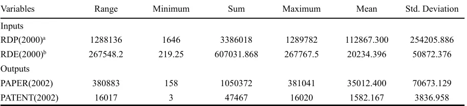
Table 1. Descriptive statistics about R&D inputs and outputs for 30 OECD countries

Variables Range Minimum Sum Maximum Mean Std. Deviation

Inputs

RDP(2000)a _{1288136 1646 3386018 1289782 112867.300 254205.886}

RDE(2000)b _{267548.2 219.25 607031.868 267767.5 20234.396 50872.376}

Outputs

PAPER(2002) 380883 158 1050372 381041 35012.400 70673.129

PATENT(2002) 16017 3 47467 16020 1582.167 3836.958

a_{It is a FTE (Full Time Equivalent) on R&D.}

b_{Its unit is million constant dollars – 2000 prices and PPPs.}

This paper uses R&D inputs and outputs with a two-year time lag for 30 OECD countries to serve the relevant quantitative analyses about presented WADD models③

. The result of

③

descriptive statistics is displayed in table 1. Evidently, the multivariable evaluation system is characterized by “multi-unit” and “disparate orders of magnitude”.

3. Review on standardization-based formulations of existing WADD models

The basic ADD model was proposed by Charnes et al. (1985), whose specific program formulation (P1) is as follows.

1 1 1 1 1 max subject to

, 1,2, , , , 1,2, , , 1, 0 . m s io ro i r n

io _j j ij i n

ro j j rj r n

j j

j i r

s s

x x s i m

y y s r s

s s                          











  , , (P1)

The ADD model is a non-radial and Pareto–Koopmans (PK) model (Cook and Seiford, 2009). The first two equation constraints in program (P1) are translation invariant④

with the help of the convexity constraint of



n_j₁j 1 (Cooper et al., 1999), because, for given any

real number di and cr, formulas (1) and (2) always hold.

1 ( ) 1 ( ), 1, 2, ,

n n

io io j j ij io i j j ij i

s x  x x d  x d i m

 

 



  



  _ , (1)

1 1 ( ) ( ), 1, 2, ,

n n

ro _j j rj ro _j j rj r ro r

s  y y  y c y c r s

 





 



    _ . (2) Consequently, negative and zero inputs or outputs can be dealt with by adding suitable constants to the affected input or output sets, with assurance that the solutions will not be affected by these translations (Cooper et al., 1999). So, the whole ADD model satisfies translation invariance. However, the sum of slacks in objective function is in-commensurable measure because of the differences in measurement units and magnitude orders of slacks, i.e., the ADD model is not unit invariant (Lovell and Pastor, 1995).

Following the property of unit invariance of transformation formulas (S1) ~ (S5), it’s may be a good solution to use a statistical data-based parameter to scale each slack which makes the sum of scaled slacks satisfy the unit invariance. Because these parameters come from practical observation data, they can be seen as objective weights embodying the

④

status/importance of slacks, which in fact serve as standardization parameters embodying information of corresponding observation data. Thus it’s nature to introduce the “weighted” ADD model (WADD), whose objective function is (O1).

1 1

max m_i w si io _rs w sr ro

    

 









. (O1)

In most practical evaluations, wi and wr are user-specified weights, which embody

managers’ preference, and are obtained through value judgment (e.g., Thrall, 1996). However, it’s difficult to subjectively judge which one of observation indicators is more important than other for the tested DMU because of the supplemental relations between them. Cooper et al. (1999) points out:

“…, it is desirable to orient these choices to more “objective” criteria so that investigators doing scientific research, for instance, will reach the same (or similar) conclusions from the same (or similar) bodies of data. For this purpose, we shall confine ourselves to “data-based weights.”

The data-based weights can embody information hiding in the difference between datasets, and the inefficiency results of WADD models with data-based weights are justifiable and objective. So WADD models with data-based weights on slacks are not only mathematically scientific but also practically applicable.

Of course, for obtaining unit invariance, the weights should be “contragredient” with weighted slacks, which means that the dimensions of weights are reciprocal of these of weighted slacks (Cooper et al., 1999). From economic meaning, weights represent the marginal worth of corresponding weighted slack. Specifically in terms of WADD, weights are associated with unit costs and unit prices of excess and shortfall slack variables (Bardhan et al., 1996), and the sum of weighted slacks is used to measure the total cost of inefficiencies. The modification by weight is to make WADD models satisfy some attractive properties by scaling slacks in order to obtain commensurable inefficiency scores.

3.1 Measure of inefficiency proportions (MIP-WADD)

When _{( )} 1

i io

w _ x  _{, ( )} 1

r ro

w₌ y  _{, the objective function of corresponding WADD model}

is

1 1

max m io s ro

i r io ro

s s

x y

 



_  



_  . (O2)

which is referred to as MIP-WADD (Cooper et al., 1999). Because the numerators and denominators in (O2) have same unit, the (O2) satisfies unit invariance. However, MIP-WADD doesn’t satisfy translation invariance and suffers from zero and negative data as traditional ADD.

The unequal relationship sio xio for i must hold, but the unequal relationship ro ro

s _ y _{for r aren’t always true. So, the upper bound of inefficiency score obtained from}

MIP-WADD possibly exceeds unity, and, similarly, the average⑤

inefficiency score can’t be limited in [0, 1], i.e., can’t satisfy the sense of common (in)efficiency.

Besides, in (O2), weights _{( )} 1

i io

w _ x  _{and ( )} 1

r ro

w₌ y  _{vary with the tested DMU}

0,

which can be referred to as “weight instability”, so that the ranking of inefficiency measure generated by MIP-WADD may be considered not comparable due to the absence of a common weight for specific observation indicator. In fact, there are differences in unit costs and unit prices of surplus and shortfall slacks for different DMUs, so the unstable weights are, to a certain degree, reasonable in many practical environments.

3.2 WADD with sum-based weight (SUM-WADD)

Ali et al. (1995) also tried to introduce new weights 1 1 ( n )

i _j ij

w x  





, 1

1 ( n )

r _j ij

w y  





, where the corresponding objective function is

1 1

1 1

max m io s ro

n n

i r

ij ij

j j

s s

x y

 _  _ 

 













. (O3)

The WADD model with (O3) is referred to as SUM-WADD. The objective function (O3) is the same to (O2) in such key properties as unit and translation invariance. Although it suffers from zero data less possibly than (O2), it can’t satisfy some extreme situations, where

1 0

n ij j x 



or



n_j₁yij 0 may be exist. However, compared with (O2), the objective

function (O3) provides a common stable weight, and makes inefficiency score reduced into [0, 1].

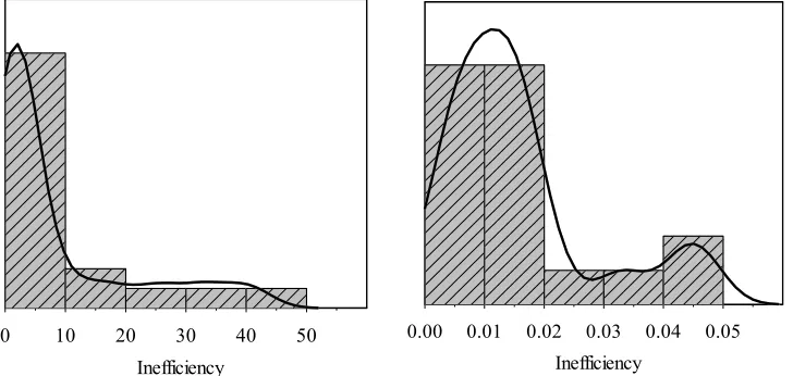
In the light of the estimated density distribution of inefficiency scores (excluding zero scores) of WADD models with (O2) and (O3) by kernel density estimation (Wand and Jones,

⑤

Usually, _



_im_（₁ s x_io* _io）



s_r（₁ s y_ro* _ro）（_ m s ） (Bardhan et al., 1996; Cooper et al., 1999) or

* *

1 1

1995; Simonoff, 1996) (Fig. 1 and Fig. 2) ⑥

, it’s easy to find that the variance between two distribution illustrations of inefficiency scores is clear. The inefficiency scores from SUM-WADD mainly converge into (0, 0.02), but majority inefficiency scores from MIP-WADD rang in (0, 10). Clearly, the congestion of inefficiency scores is very serious for SUM-WADD. A common shortcoming of both MIP-WADD and SUM-WADD is that their density function figures are very sharp in a relative smaller range of inefficiency scores against a whole range of inefficiency scores, meaning crowdedness of majority inefficiency scores and shortness of discrimination power.

0 10 20 30 40 50

Inefficiency

0.00 0.01 0.02 0.03 0.04 0.05 Inefficiency

Fig. 1. Kernel density estimation of inefficiency for

MIP-WADD Fig. 2. Kernel density estimation of inefficiency forSUM-WADD

3.3 Range adjusted measure (RAM-WADD)

Among the exiting typical WADD models, NOR-WADD and RAM-WADD can satisfy unit and translation invariance simultaneously.

In a working paper (Cooper and pastor, 1995), RAM-WADD is proposed, which can be also found in Cooper et al. (1999).

Here, ₍ U L₎ 1

i i i

w _ x _x  _{, (} U L₎ 1

r r r

w₌ y _y  _{, so the objective function of RAM-WADD is}

1 1

max m io s ro

U L U L

i r

i i r r

s s

x x y y

  _{ }   _  _

 







. (O4)

Because,

( U ) ( L ) U L i i i i i i

x d  x d x x and ( U ) ( L ) U L r r r r r r

y c  y c y y ,

hold for i r j, , , (O4) is translation invariant (Cooper et al., 1999). However, as shown in the

⑥

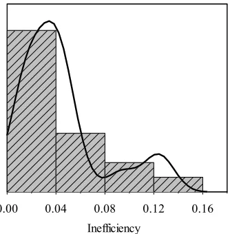
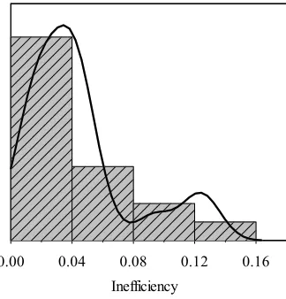
[image:11.612.130.494.239.412.2]

[image:12.612.224.391.145.315.2]

Fig. 3, the inefficiency scores obtained from RAM-WADD mainly converge into (0, 0.04). This is mainly due to big differences between maximum and minimum within the dataset, which causes weights too small. Inefficiency congestion in SUM-WADD is attributable to the same reason.

0.00 0.04 0.08 0.12 0.16 Inefficiency

Fig. 3. Kernel density estimation of inefficiency for RAM-WADD

3.4 Standardized additive DEA (NOR-WADD)

Another inefficiency measure which satisfies translation invariance is NOR-WADD,

which was proposed by Lovell and Pastor (1995).

Here, _{( )} 1

i i

w _   _{, ( )} 1

r r

w₌  _{, and the objective function is}

1 1

max m io s ro

i r i r

s s



 

 

   

 

 _  _







. (O5)

Because,













2





2

1 1 1 1

n n

ij i i i ij i i j x d x d n j x x n 



       



＝



＝ and













2





2

1 1 1 1

n n

ij r r r ij r r j y c y c n j y y n 



       



＝



＝

hold for any given constant di and cr, i r j, , , (O5) is translation invariant. Comparing

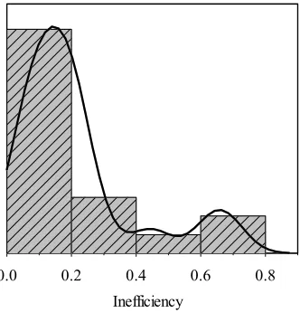
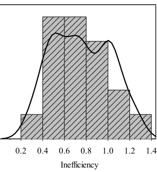
[image:12.612.85.490.432.590.2]

[image:13.612.230.396.63.236.2]

0.0 0.2 0.4 0.6 0.8 Inefficiency

Fig. 4. Kernel density estimation of inefficiency for NOR-WADD

3.5 Rang of improvement measure (RIM-WADD) ⑦

Besides, Pastor (1994) proposed another inefficiency measure model from the range of possible improvement in each observation indicator (input or output) for DMU0(Pastor and

Ruiz, 2007) (referred to asRIM-WADD).

Because n ₁ L

io io j j ij io i

s x  x x x







 

＝ and

1

n _U

ro j j rj ro r ro

s  y y y y







   hold for

, ,

i r j

 _{, if let} *

io

x and *

ro

y be contributing inputs and obtained outputs in practical

production process, then io* io io* L L io i io i

s x x

x x x x

 _ 

  show the rate of the rang of practical surplus *

io io

x x (potential improvement, i.e., inputs contraction) to the range of possible maximum

surplus L

io i

x x , and ro* *ro ro

U U r ro r ro

s y y

y y y y

 _ 

  show the rate of the rang of practical shortfall *

ro ro

y y (potential improvement, i.e., output expansion) to the range of possible maximum shortfall U

r ro

y y .

So for RIM-WADD, ₍ L₎ 1

i io i

w _ x _x  _{, (} U ₎ 1

r r ro

w _ y _y  _{, i.e., the objective function is}

1 1

max m io s ro

L U

i r

io i r ro

s s

x x y y

  _{ }   _  _

 







. (O6)

Because ( ) ( L ) L

io i i i io i

x d  x d x x and ( U ) ( ) U r r ro r r ro

y c  y c  y y hold fori r j, , , where di and cr are any given constant numbers, (O6) also satisfies translation

invariance. But, (O6) easily suffers from zero data, because L io i

x x and U ro r

y  y always

⑦

exist.

[image:14.612.232.389.81.253.2]

0.2 0.4 0.6 0.8 1.0 1.2 1.4 Inefficiency

Fig. 5. Kernel density estimation of inefficiency for RIM-WADD

Another problem associated with RIM-WADD is that it is an inefficiency measurement with unstable weights, which is the same to MIP-WADD. However, inefficiency scores generated by it most lie in a larger bounded range (0.4, 1.0) (see Fig. 5), which shows a better power in inefficiency discrimination than SUM-WADD, NOR-WADD and RAM-WADD.

3.6 Brief summary and discussion

Firstly if visually compare the formulas for standardization with the formulations of objective functions of WADD, it’s evident that there are corresponding relationships mainly in denominators, such between (S1) and (O5), between (S3) and (O4) as well as between (S5) and (O3). Although, there are no corresponding standardization formulas for (O2) and (O6), we can use their denominators to scale observation datasets for convenient calculation.

Specifically comparing denominators of objective functions (O2) ~ (O3) with (O4) ~ (O6), clearly their formulations are different. The former is a single statistic (including specific observation data, hereafter), however the latter is a difference between two statistics which makes denominators are stable when two statistics add or reduce a constant simultaneously. If let ( )a

i

S v and ( )b i

S v standard for the two different statistics (maximum, minimum or mean) of all observation values in the dataset vi, when adding a constant di to the dataset vi, then

( )a ( )b ( ( )a ) ( ( )b ) ( )a ( )b

i i i i i i i i i i

S v d S v d  S v d  S v d S v S v _.

observation dataset is the difference form in itself. Moreover, considering the constraints in (P1), then

1

n _{L U L} io io _j j ij io i i i

s x  x x x x x



 



     ( L) 1

io io i

s x _x _{ and (} U L_{) 1} io i i

s x _x _{ ,}

1 ( ) 1

n _{U U L U}

ro _j j rj ro r ro r r ro r ro

s  y y y y y y s y y







        and ( U L) 1

ro r r

s y _y _{ .}

The formations of (O4) and (O6) mainly depend on these equivalences, clearly which ensure the objective function values of WADD models range in [0, 1] with a multiplier1 m s . But WADD models with (O2) and (O5) can’t ensure that (in)efficiency scores are below unity, so (O4) and (O6) have more superiority than them in satisfying the sense of (in)efficiency.

Besides, for (O3), (O4) and (O5), w_i _and

r

w _{don’t vary from one DMU to another.}

However, for (O2) and (O6), wi and wr vary from one DMU to another because of the

impact of specific observation. This means that the weights in (O2) and (O6) are unstable. Cooper et al. (1999) meant that (in)efficiency results based on unstable weights can’t be used as ranking comparison. Even in the case of (O5), it’s not always suitable for all evaluation principles, because the numerators and denominators would be measuring distances from different points—with the standard deviations measuring distance from the mean, while the slack values would be measuring distance from a point on the boundary of the observations (Cooper et al., 1999).

4. New extensions of WADD models based on two standardization techniques

4.1 WADD with maximum as weight (Max-WADD)

In many practical statistical analyses, the maximum in a observation dataset usually is used to scale all observation data, i.e., normalizing the original dataset by (S2), in order to make all observation datasets reduced into a commensurable range [0, 1] when original observation data are not negative. So, the objective function of corresponding Max-WADD model can be formulated as (O7) as follows.

1 1

max m io s ro

U U i r

i r

s s

x y

  _{ }   _  _







. (O7)

Evidently, _{( )}U 1

i i

w _ x  _{and ( )}U 1

r r

w _ y  _{. The attractive properties of (O7) can be interpreted}

form two aspects. One aspect is that U 1

io i

s x _{ and} U ₁ ro ro

s y _{ can make  bounded not}

exceed unity with a multiplier1 m s , and the other is that _U n ₁ i _j ij

x 



_ x  and _U n ₁ r _j ij

y 



_ y

make (O7) generate larger proportions than (O3) at least.

[image:16.612.223.385.368.537.2]

0.00 0.04 0.08 0.12 0.16 Inefficiency

Fig. 6. Kernel density estimation of inefficiency for Max-WADD

Although U L U

i i i

x x x and U L U r r r

y y  y , the inefficiency distribution in Fig. 6 shows that the inefficiency result of Max-WADD is almost the same to that of RAM-WADD. The coincidence also can be proved by the empirical datasets in Aida et al. (1998), which is mainly due to the large difference between maximum and minimum.

4.2 WADD with mean as weight (Mean-WADD)

different orders of magnitude of datasets (xij and yrj) for different production scales (as the

results in Aida et al. (1998)), there is a big difference between some statistics such as sum, maximum as well as range and majority observation data within the dataset, so weights coming from reciprocals of sum, maximum and range must be smaller. This causes a smaller (in)efficiency score. So for obtaining a better power in (in)efficiency discrimination in terms of frequently-used statistics available, we can let _{( )} 1

i i

w_ x  _{and ( )} 1

r r

w_ y  _{, then the}

corresponding objective function is

1 1

max m io s ro

i r i r

s s

x y

  _{ }   _  _







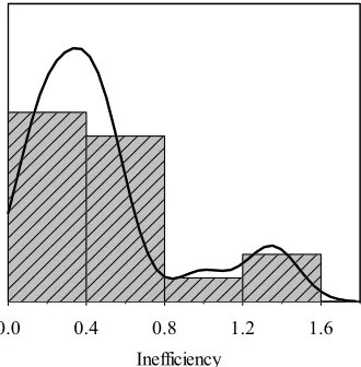
. (O8)

Fig. 7 depicts the density distribution of inefficiency scores based on WADD with (O8). Although it is the similar distribution shape to Fig. 3 depicting inefficiency results from SUM-WADD, the range of inefficiency scores expands much (from (0, 0.05) to (0, 1.6) ), showing a better distinction power in inefficiency results.

[image:17.612.225.390.360.528.2]

0.0 0.4 0.8 1.2 1.6 Inefficiency

Fig. 7. Kernel density estimation of inefficiency for Mean-WADD

5. An empirical comparison of (in)efficiency discrimination power

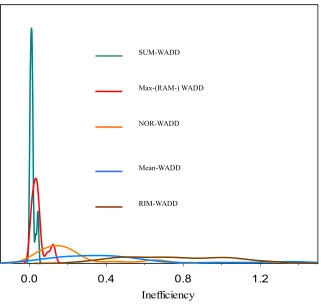
By Splus 9.0, the comparison result⑧

of Kernel density estimations of inefficiency scores for WADD models with (O3) ~ (O8) gives a complete comparison in inefficiency discrimination power, which is SUM-WADD< RAM (Max)-WADD< NOR-WADD <Mean-WADD < RIM-WADD as shown in Fig. 8.

⑧

0.0 0.4 0.8 1.2

[image:18.612.146.467.57.361.2]

Inefficiency

Fig. 8. Comparing Kernel density estimations of inefficiency for (O3) ~ (O7)

Note: The efficiency is calculated by authors associated with Excel solver

Besides, in order to maintain the inefficiency level “_*_{” being on the unit scale [0, 1], a}

constant  is introduced to balance



_im₁w si io 



_rs₁w sr ro  , i.e.,



1 1



max m_i w si io s_r w sr ro

     

 

 







_.

So, if 0_w s_{i io}  _1 _{and 0 1}

r ro

w s 

  , and let  1 (m s) , then _*_{[0,1] as a}

measure of inefficiency satisfying the sense of inefficiency. At the same time, a measure of efficiency, _*_{=1 }* _{[0,1], is obtained, which satisfies the sense of efficiency. Obviously,}

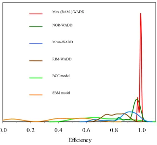
RAM-WADD, Max-WADD and SUM-WADD can satisfy the condition. In fact, Mean-WADD and NOR-WADD with  1 (m s) can satisfy the condition under general environments. The Fig. 9 displays a complete comparison of Kernel density estimations of efficiency scores for WADD models with (O5) ~ (O8) including BCC and SBM (Tone, 2001). Obviously, in discrimination power, BCC (SBM)> RIM-WADD >Mean-WADD > NOR-WADD > RAM/Max -WADD. The efficiency range of BCC and SBM not only is wider, but also distribution curve is not sharp, meaning that efficiency distribution is not centralized

NOR-WADD Max-(RAM-) WADD

Mean-WADD SUM-WADD

and has a better discrimination power.

0.0 0.2 0.4 0.6 0.8 1.0

[image:19.612.146.465.86.381.2]

Efficiency

Fig. 9. Comparing Kernel density estimations of efficiencies for (O5) ~ (O8) including BCC and SBM

Note: The efficiency is calculated by authors associated with Excel solver except for BCC efficiency

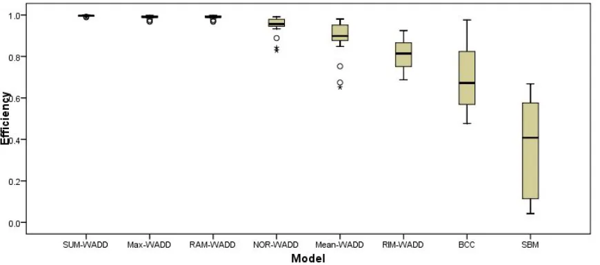
Fig. 10 provides another illustration for efficiency distribution and discrimination power of WADD models with (O3) ~ (O8) including BCC and SBM by a boxpolt, which displays a visual comparison of the variation of efficiency scores across those models. Evidently, the variation of efficiency scores yielded by all WADD models is less than that from BCC and SBM, and Mean-WADD yields a bigger variation than SUM-WADD, Max-WADD, RAM-WADD and NOR-WAD. Among WADD models, the RIM-WADD yields the lowest average efficiency, and there is no visual difference in the average efficiency from SUM-WADD, Max-WADD and RAM-WADD.

SBM model BCC model RIM-WADD NOR-WADD

[image:20.612.91.526.62.254.2]

Fig. 10. Comparing efficiency estimates for (O3) ~ (O8) including BCC and SBM

Note:The median for each dataset is indicated by the black centre line (i.e. where 50% of the data is above it and 50% below it). The first and third quartiles of the data are at the edges of the grey box where, respectively, 25% of the data falls below it and 25% of the data is above it. The total length of the grey box is known as the inter-quartile range (IQR). The extreme values (within 1.5 times the inter-quartile range from the upper or lower quartile) are the ends of the lines (or whiskers) extending beyond the grey area. Points that lie at a greater distance from the median than 1.5 times the IQR are plotted individually and may be regarded as outliers.

There is tradeoff between the sense of (in) efficiency with respect to making _*

satisfying [0, 1] and the discrimination power. Obviously, the bigger values of wi and r

w _{are needed. However, this always causes inefficiency crowed, which means that some}

measure formulations are mathematically acceptable but practically unacceptable (Sueyoshi and Sekitani, 2009).

6. Applications

Since this study has related the formulation of WADD models to the standardization of original datasets, it’s helpful for users to flexibly apply various WADD models to heterogeneous original datasets and facilitate users’ calculations. Furthermore, the attractive translation property of some WADD models helps in improving the formulation of DEA-based hybrid measure model in the presence of zero and negative values.

6.1 Smoothing WADD models’ calculation

If wi and wr come from the statistics of observation datasets, when observation

1 1 1 1 1 max subject to

, 1,2, , , , 1,2, , , 1,

0 .

m s i io r ro i r n

io j j ij i n

ro _j j rj r n

j j

j io ro

w s w s

x x s i m

y y s r s

s s                            











  , , (P2)

Because w_i _and

r

w _{are non-zero constants for given sample observation datasets,}

then

1

1

n , 1,2, ,

n

io _j j ij io i io j i ij i io j

x  x s w x  w x w s  i m









  ＝



  _{ ,}

1 1 , 1, 2, , .

n n

ro _j j rj ro r ro _j j r rj r ro

y  y s w y  w y w s  r s

 





  ＝



  

If let sˆ_io _w s_{i io}  _0_{, ˆ 0}

ro r ro

s _w s  _{ , ˆ}

ij i ij

x _w x _{and ˆ}

rj r rj

y _w y _{, then program (P2) can be}

changed into



1 1



1 1 1

ˆ _{max ˆ ˆ}

subject to

ˆ ˆ , 1,2, , ,ˆ

ˆ ˆ ˆ , 1,2, , ,

1, ˆ ˆ

0 , , .

m s io ro i r n

io _j j ij io n

ro _j j rj ro n

j j

j io ro

s s

x x s i m

y y s r s

s s                          











  (P3)

Comparing the original ADD model (P1) and the transformed ADD model (P3), their structures are obviously same. However, program (P3) is dimensionless in both observation

data and slacks, so the value of sum formulation * *

1ˆ 1ˆ

m s io ro i s r s

    





is commensurable,

which can be used to rank inefficiency level.

In fact, the transformation process from (P1) to (P3) is a standardization (or referred to as scaling) process of original datasets. So, it’s necessary to preprocess original datasets when using ADD model.

(P3) instead of (P2) to deal with preprocessed data for the comparable efficiency results. Based on the formulas (1) and (2), for input and output constraints, the formula set (3) holds.

1 1

1 1

( ) ( ), 1, 2, , .

( ) ( ), 1, 2, , .

n n

i io i io _j j i ij i io i _j j i ij i

n n

r ro _j j r rj r ro _j j r rj r r ro r

w s w x w x w x d w x d i m

w s w y w y w y c w y c r s

                                 









  (3)

For example, when ₍ U L₎ 1

i i i

w _ x _x  _{, (} U L₎ 1

r r r

w₌ y _y  _and L i i

d＝x , c_r＝y_rL , the formula set (4) holds for , .i r

1 1 ( ) ( ) ( ) ( ) L L

n _{ij i} io io i

j

U L U L j U L i i i i i i

L L n rj r

ro ro r

j

U L j U L U L r r r r r r

x x

s x x

x x x x x x

y y

s y y

y y y y y y

                   





(4)

When _{( )} 1

i i

w_   _{, ( )} 1

r r

w₌  _and

i i

d＝x , c_r＝y_r , the formula set (5) holds

for , .i r

1

1

( )

( )

( ) ( )

n ij i io io i

j j

i i i

n _{rj r}

ro ro r

j j

r r r

x x

s x x

y y

s y y

                         





(5)

So, if use ADD model to deal with standardized datasets by (S1) or (S3), the inefficiency results are the same to them from NOR-WADD or RAM-WADD. This is more interpretive and convenient calculated than NOR-WADD or RAM-WADD.

Remark 2: Before using WADD, one can standardize the original observation data directly using (S1) ~ (S5) according to the corresponding formulation of objective function of WADD. The standardized data can be dealt with by ADD which doesn’t damage the inefficiency results directly generated by WADD.

This conclusion is supported by Ali et al. (1995). They concluded as follows:

“…….It follows that caution should be exercised in selecting units of measurement if the

standard model is to be used without manipulation of the data. To fully ‘standardize’ the model and prevent the inappropriate aggregation of non-commensurable measures, some preprocessing of data may be required.”

6.2 Improving multi-stage models

on the slacks generated from the BCC-DEA model. It is very attractive and used in many practical fields, such as bank efficiency (Liu and Tone, 2008), R&D efficiency (Wang and Huang, 2007), transit efficiency (Margari et al., 2007) and public institutes efficiency (Glass et al., 2006). The essential contribution of multi-stage model is to generate a “pure” measure for technical efficiency removing the compact of environment factors and stochastic noise, which makes all DMUs compared each other in a common environment and common luck scenario.

However, there are limitations and shortcomings for the multi-stage efficiency measure model. Firstly, in view of the inability dealing with negative and zero values for radial BCC-DEA model due to not being translation invariant, Fried et al. (1999, 2002) has to have proposed adjusted formulations only by adding the difference between maximum predicted slack and predicted slacks on the original inputs and outputs. Besides, BCC slacks adopted in Fried et al. (1999, 2002) are not unit invariant (Lovell and Pastor, 1995) or commensurable. And, BCC model ignores the role of slacks in calibrating the efficiency score, thus measured efficiency allows for upward bias (Liu and Tone, 2008; Cooper et al., 2005). Furthermore BCC slacks are divided into radial and non-radial slacks, which gives rise to concern that some useful information could be lost (Liu and Tone, 2008).

Although Liu and Tone (2008) and Avkiran (2009) proposed new multi-stage measure models based on the SBM model with unit invariance, it still can’t deal with negative and zero data due to the shortness of translation invariance in SBM. So, for avoiding the negative and zero values, their adjusted processes still accounted for least favorable operating environment for inputs slacks (most favorable operating environment for output surpluses) and didn’t incorporate the most favorable and average operating environments into efficiency measuring.

So an enhanced multi-stage model for making up shortcomings above is necessary. RAM-WADD, RIM-WADD or NOR-WADD has more attracting properties than both BCC model used in Fried et al. (1999, 2002) and SBM model used in Liu and Tone (2008) and Avkiran (2009), which can simultaneously measure the radial and non-radial efficiency and accommodate negative and zero values due to unit and transformation invariance.

slacks are obtained due to the property of unit-invariance of the chosen WADD model. Then users use stochastic frontier analysis (SFA) to regress those standardized slacks against a set of context variables with consideration of three effects: operating environmental effects, managerial inefficiency, and statistical noise. In the third stage, users adjust standardized inputs or outputs in a manner that accounts for the environmental effects and the statistical noise uncovered in the second stage, and subsequently repeat the first stage analysis by applying the chosen WADD model to the adjusted standardized datasets. A new multistage model for pure efficiency measures, WADD-SFA-WADD, is formed. In our analytical framework, one can adjust original input and output datasets from average, favorable or unfavorable operating environments.

6.3 Brief summary and discussion

It’s necessary to standardize original datasets by given transformation formulas in this paper for making them dimensionless and commensurable, or to use corresponding WADD models directly. It’s inevitable that there is much heterogeneity in a multivariable evaluation environment, which usually embodies variances in units of measurement across datasets and orders of magnitude within one dataset. So, it’s not advisable to aggregate the slacks with heterogeneous measure units directly by sum. Though pre-standardization process by standardization formulas, WADD models with descriptive statistics-based weights can be transformed into the traditional ADD model, the sum of whose slacks can stand for inefficiency level.

Because the constraints of (weighted) additive DEA models meet unit and translation invariance, what one need do is to make objective functions meet the two desirable properties by adding proper weights on slacks. The “statistical data-based” weights should be chosen for a fair and objective comparison. Moreover, the chosen weights should make the value of objective function satisfy a clear discrimination power for comparison requirements, i.e., the formulation of weighted objective function should be mathematically and practically acceptable.

that Mean-WADD and NOR-WADD usually perform well, and RIM-WADD performs most out of existing WADD models in terms of distribution of (in) efficiency scores.

[image:25.612.79.534.311.445.2]

Of course, the empirical choice of WADD models is not random. Table 2 summarizes the comparisons among the objective functions of seven WADD models in terms of the standardization techniques as well as six properties including (in)efficiency judgment, unit invariance, translation invariance, stability of weight with respect to being invariable or variable for any DMU, sense of (in)efficiency and discrimination power. Table 2 provides us with the fact that none of relevant seven WADD models show a better performance for all six properties. All WADD model perform well in (in)efficiency judgment and unit invariance, but display a inconsistent performance in other four properties. So, decision-makers should choose suitable WADD models depending on the need of specific decision environments.

Table 2. Summary on properties of seven WADD models

Measure model _-WADDMIP _-WADDRAM _-WADDNOR _-WADDSUM _-WADDRIM _-WADDMax _-WADDMean Standardization

formula-based Noa (S3) (S1) (S5) (S3) or (S3)* (S2) (S4)

(In)efficiency judgment Yes Yes Yes Yes Yes Yes Yes

Unit invariance Yes Yes Yes Yes Yes Yes Yes

Translation invariance No Yes Yes No Yes No No

Stability of weight No Yes No Yes No Yes Yes

Sense of (in)efficiencyb _{No Yes No Yes Yes Yes No}

Discrimination powerc _{Good Bad Relative good Very bad Very good Bad Good} a_{MIP-WADD corresponds to the standardization approach of using the evaluated input and output to scale all inputs and}

outputs.

b_{The sense of (in)efficiency of WADD is obtained associated with scale parameter 1 (m s) .} c_{Discrimination power is based on the distribution of (in)efficiency values associated with Splus 9.0.}

Note: (a) “Yes” indicates that a WADD model satisfies a desirable property and “No” indicates an opposite case.

(b) MIP-WADD in Cooper et al. (1999) or Sueyoshi and Sekitani (2009); RAM-WADD in Cooper et al. (1999); NOR-WADD in Lovell and Pastor (1995); SUM-WADD in Ali et al. (1995) or Thrall (1996); RIM-WADD in Pastor (1994); Max-WADD and Mean-WADD in section 4 of this study.

Finally, RAM-WADD, NOR-WADD and RIM-WADD satisfy unit and translation invariance simultaneously, which can deal with negative and zero values. So, they inspire a motivation to improve multi-stage efficiency measure in Fried et al. (1999, 2002) for conquering the negative impact of unit variances of slacks on the efficiency comparison and allowing one to adjust original input and output data from average, favorable or unfavorable operating environments.

7. Conclusion

desirable properties of weighted additive DEA (WADD) associated with the standardization methodologies of original observation datasets. The main purpose of our investigations is to facilitate the applications and extensions of WADD models for users in terms of reasonable interpretations and convenient calculation.

In this study, the formulations of objective functions of weighted additive DEA (WADD) models are endowed with a practical statistical background, which are novelly related to the standardization of orginal observation datasets, and make WADD models meet the interpretive requirements. It’s proved that the preprocessing of original datasets by standardization formulas before using tradiational ADD model is the consistent with directly applying the corresponding WADD models. Depending on the translaiton invariance property of some WADD models, this study propose a new multistage model for pure efficiency measures, WADD-SFA-WADD. By the new hybrid model as an improved analytical framework of Fried et al. (1999, 2002), one can adjust original input and output datasets from average, favorable or unfavorable operating environments.

In terms of future work, our investigations in this study can be applied to various empirical applications. Moreover, it’s practically valuable to implement more empirical and theoretical comparisons among WADD models, and investigate more evidences for the choice of WADD models in different evaluation contexts. Especially in the discrimination power of (in)efficiency scores, our rough conclusions in table 2 need more evidences as a future special research task before reaching a general rule.

Reference:

Aida K, Cooper WW, Pastor JT, Sueyoshi T (1998). Evaluating Water Supply Services in Japan with RAM–—A Range-Adjusted Measure of Inefficiency. Omega 26:207-232.

Ali AI, Lerme CS, Seiford LM (1995). Components of efficiency evaluation in data envelopment analysis. European Journal of Operational Research 80: 462-473.

Ali AI, Seiford, LM (1990). Translation invariance in data envelopment analysis. Operations Research Letters 9:403-405.

Avkiran NK (2009). Removing the impact of environment with units-invariant efficient frontier analysis: An illustrative case study with intertemporal panel data. Omega, 37:535-544.

Banker RD (1984) Estimating most productive scale size using data envelopment analysis. European Journal of Operational Research 17:35-44.

in DEA. Part I: Additive Models and MED Measures. Journal of the Operations Research Society of Japan 39:322-332.

Charnes A, Cooper WW, Golany B, Seiford L, Stutz J (1985). Foundations of Data Envelopment Analysis for Pareto-Koopmans efficient empirical production functions. Journal of Econometrics 30:97-107. Charnes A, Cooper WW, Rhodes E (1978). Measuring the efficiency of decision making units. European

Journal of Operational Research 2:429-444.

Cook WD, Seiford LM (2009). Data envelopment analysis (DEA) – Thirty years on. European Journal of Operational Research 192:1-17.

Cooper WW, Park KS, Pastor JT (1999). RAM: A Range Adjusted Measure of Inefficiency for Use with Additive Models, and Relations to Other Models and Measures in DEA. Journal of Productivity Analysis 11:5-42.

Cooper WW, Pastor JT, Aparicio J, Pastor D (2011).BAM: a bounded adjusted measure of efficiency for use with bounded additive models 2:85-94.

Cooper WW, Seiford LM, Tone K, Zhu J (2007). Some models and measures for evaluating performances with DEA: past accomplishments and future prospects. Journal of Productivity Analysis 28:151-163. Fried HO, Lovell CAK, Schmidt SS, Yaisawarng S (2002). Accounting for environmental effects and

statistical noise in data envelopment analysis. Journal of Productivity Analysis 17:157-174.

Fried HO, Schmidt, SS, Yaisawarng S (1999). Incorporating the operating environment into a nonparametric measure of technical efficiency. Journal of Productivity Analysis 12:249-267.

Glass JC, McCallion G, McKillop DG, Stringer K (2006). A ‘technically level playing-field’ profit efficiency analysis of enforced competition between publicly funded institutions. European Economic Review 50:1601-1626.

Liu J, Tone K (2008). A multistage method to measure efficiency and its application to Japanese banking industry. Socio-Economic Planning Sciences 42:75-91.

Lovell CAK, Pastor JT (1995). Units invariant and translation invariant DEA models. Operations Research Letters 18:147-151.

Margari BB, Erbetta F, Carmelo P, Piacenza M (2007). Regulatory and environmental effects on public transit efficiency: a mixed DEA-SFA approach. Journal of Regulatory Economics 32:131-151.

Pastor JT (1994). New Additive Models for Handling Zero and Negative Data. Working Paper, Departamento de Estadistica e Investigacion Operativa, Universidad de Alicante, Spain.

Pastor JT (1996). Translation invariance in data envelopment analysis: A generalization. Annals of Operations Research 66:93-102.

Pastor JT, Ruiz J (2007). Variables With Negative Values In Dea. In: Zhu J, Cook WD. (Eds.) Modeling Data Irregularities and Structural Complexities in Data Envelopment Analysis. Springer, New York. Simonoff JS (1996). Smoothing Methods in Statistics. Springer, New York.

Journal of Operational Research 196: 764-794.

Thrall RM (1996). Duality, classification and slacks in DEA. Annals of Operations Research 66: 109-138. Tone K (2001). A slacks-based measure of efficiency in data envelopment analysis. European Journal of

Operational Research 130:498-509.

Wand MP, Jones MC (1995). Kernel Smoothing. Chapman and Hall, London.