What Does Crypto currency Look Like? Gaining Insight into Bitcoin Phenomenon

(1)

Munich Personal RePEc Archive

What Does Crypto-currency Look Like?

Gaining Insight into Bitcoin Phenomenon

Bouoiyour, Jamal and Selmi, Refk

CATT, University of Pau, France, ESC, University of Manouba,

Tunisia.

26 August 2014

Online at

https://mpra.ub.uni-muenchen.de/58133/

(2)

WHAT DOES CRYPTO-CURRENCY LOOK LIKE?

GAINING INSIGHT INTO BITCOIN PHENOMENON

JAMAL BOUOIYOUR CATT, University of Pau, France. E-mail: jamal.bouoiyour@univ-pau.fr

REFK SELMI

ESC, University of Manouba, Tunisia. E-mail: s.refk@yahoo.fr

Abstract: The present paper seeks to effectively address the following question: What Bitcoin looks like? To do so, we regress Bitcoin price on a number of variables (Bitcoin fundamentals recorded in the literature) by applying an ARDL Bounds Testing approach for daily data covering the period from December 2010 to June 2014. Our findings highlight the speculative nature of Bitcoin. We also provide insightful evidence that Bitcoin may be used for economic reasons but there is any sign of being a safe haven or a long-term promise. By considering the Chinese trading bankruptcy, the contribution of users‟ interest stills sharply dominant, highlighting the robustness of our results.

(3)

1. Introduction

Since its creation in 2009 by Satoshi Nakamoto-pseudonym, the Bitcoin has experienced multiple peaks and successive ups and downs. Is it a safe haven or a speculative trap? Is it a short-term hedge? Is it a poor long-term investment or a long-run promise? The opinions about this nascent currency have drawn a substantial attention from investors, advisers and market regulators. The fact that questions get frequently and heavily asked indicates the very prime importance of this phenomenon.

Bitcoin is virtual money with zero intrinsic value issued by computer code in electronic portfolios, which is not convertible into anything and not have the backing of any Central Banks and any government. The value of a Bitcoin is neither a convertible tangible asset (such as gold) nor a fiat currency (such as dollar). It is determined by the interplay of supply and demand. This nascent crypto-currency fulfills various functions. It facilitates business transactions from person to person worldwide without any intermediary, reduces trade barriers and increases the productivity. Nevertheless, Bitcoin remains far from certain because of its sizeable price volatility, the inelastic money supply coded by mathematic formula and the lack of legal security. Bitcoin is a digital currency in a nascent stage closely associated to multiple risks stemming from its extra volatility and its speculative nature.

Despite its sharp popularity, there still very few works analyzing Bitcoin phenomenon. These researches seem insufficient to appropriately address the huge amount of questions around it. For instance, the study of Kristoufek (2013) focuses only on assessing whether

Bitcoin is a “speculative bubble” by exploring the link between Bitcoin and users‟ interest. In

addition, Glaser et al. (2014) have attempted to evaluate if Bitcoin is an asset or a currency. Besides, Kristoufek (2014) has tried to investigate whether Bitcoin is more driven by technical, financial or speculative factors by applying coherence wavelet. This technique allows it to consider the interconnection between each two variables without considering the possible interaction with other time series. In other words, this analysis is incomplete and may lead to biased results. More accurately, wavelet coherence may not be considered usually as perfect technique. On the one hand, it may lead to confuse outcomes since the occurrence of noise cannot be heavily neglected, disrupting then the studied relationship (Ng and Chan, 2012). On the other hand, wavelet decomposition is generally applied to assess the periodicity and the multiple signals that happen over time. Moreover, when we consider only two variables in wavelet analysis, we generally fall on the problem of simple regression without control variables. This highlights the inability of this technique to capture proper and accurate outcomes since it may distort the estimate. In that context, Aguiar-Conraria and Soares (2011) argue that the findings change intensely when we move from wavelet investigation with two variables for conditional wavelet estimation (with more than two variables or by adding other explanatory time series). This implies that the use of large-scale parameters of each two

variables as the case of Kristoufek (2014)‟s study may prompt inconclusive results in terms of

the interaction dynamic between Bitcoin price and its main drivers. This reinforces the need to take into account the control variables to confirm the obtained findings.

Due to the complexity of this new digital currency, the Bitcoin phenomenon demands a deeper investigation. Hence, the present paper attempts to address several questions in order

(4)

safe haven or a speculative trap? Is it a business income? Is it a short-term hedge? Is it good idea to invest in Bitcoin? Is it a long term promise?

To find better paths, our contribution to this debate is to check the robustness of the previous results and to answer further questions by adding additional explanatory variables and by carrying out convenient method that considers the interaction dynamic between several variables and captures the shocks of own series with others. To this end, we regress Bitcoin price on investors‟ attractiveness, exchange-trade volume, monetary Bitcoin velocity, estimated output volume, hash rate, gold price and Shangai market index. We apply an ARDL Bounds Testing approach, innovation accounting by simulating variance decomposition and impulse response function and VEC Granger causality test for daily data for the period spanning between December 2010 and June 2014.

We show interesting outcomes: In the short-run, the investors attractiveness, the exchange-trade ratio, the estimated output volume and the Shangai index affect positively and significantly the Bitctoin price, while the monetary velocity, the hash rate and the gold price have no influence. In the long-run, the speculative nature of Bitcoin, the output volume and the Chinese stock market index have no significant effect on Bitcoin price, while the hash rate explains significantly the dynamic of this new virtual currency. The influence of exchange-trade ratio becomes less strong, whereas the effects of the monetary velocity and the gold price still insignificant in the long term. These findings appear solid and unambiguous since there is a very slight change when incorporating a dummy variable relative to the bankruptcy of Chinese trading company. The inclusion of additional variables which have no great influence on Bitcoin price development (oil price, Dow Jones index and a dummy variable denoting the closing of Road Silk by FBI) has led to unstable estimates. Beyond the nuances of short and long terms, this research confirms the speculative nature of Bitcoin and its partial usefulness in economic reasons without forgetting the utmost importance of accounting for Chinese stock market and the processing power of Bitcoin network when analyzing the Bitcoin price dynamic. This new digital money seems far from being a safe haven and a long-term promise.

The remainder of the article proceeds as follows: Section 2 presents a brief literature survey. Section 3 describes our data and presents our methodological framework. Section 4 reports our main results and discusses them. Section 5 focuses on robustness check. Section 6 concludes and offers policy implications that may be fruitful for investors and regulators.

2. Brief literature survey

Bitcoin has engaged the attention of Medias and researchers, acknowledging the complexity of this new digital currency. Some researchers considered Bitcoin as financial instrument rather than currency or payment system. Others called it “evil” since it is not

controlled nor by central banks nor by governments. Some economists defined it as “a

speculative trap” because of its extreme volatile behavior (Buchholz et al. (2012), Kristoufek

(5)

argue that “economists scoffed at Bitcoin as more of a financial experiment than a legitimate payment system. Some economists denounced it as evil, because its value is not backed by any government nor can it be used to make pretty things as can gold. Others show that with no

intrinsic value, Bitcoin‟s rising price constituted a speculative bubble”.

The study of Kristoufek (2014) attempts to determine whether Bitcoin is likely to be safe haven, speculative bubble or transactions tool by analyzing the potential sources of Bitcoin price fluctuations including supply-demand fundamentals, speculative and technical drivers. Wavelet coherence has been carried out to investigate properly and effectively the evolution of correlations between the considered variables at different time frequencies. The obtained results reveal that the fundamental factors such as exchange-trade ratio play substantial roles in the long-run (short frequencies). The Chinese index seems an important source of Bitcoin price evolution, while the contribution of gold price dynamic appears minor and sometimes unclear. He finds also that Bitcoin prices are mainly influenced by investors‟ interest and thus by the speculative behaviors of businesses. This interconnection is most dominant at lower frequencies (higher time scale). Intuitively, the findings reveal that during

the explosive prices period, the investors‟ attractiveness to this nascent currency drives this

currency price up, while it drives it down during rapid declines period.

Glaser et al. (2014) have tried to address what intentions are businesses and investors following when moving their currency‟s usage from domestic ones into a crypto-currency like Bitcoin. By applying an Autoregressive Conditional Heteroskedasticity model, they show that the motivation of investors to Bitcoin and their intention to gather proper and additional information about its development has a great effect on this crypto-currency exchange volume, while the nexus between Bitcoin and users‟ interest seems insignificant when considering the volume within the Bitcoin system. These observed outcomes may be owing to the fact that exchange users prefer usually to keep their Bitcoins in their exchange wallet to avoid speculation and cyber-attacks without any intention to use them in economic reasons (trade transactions, for example).

Bouoiyour et al. (2014) attempt to appropriately address whether Bitcoin is a business income or risky investment. They use Granger causality to assess the relationship between Bitcoin price and exchange-trade ratio to answer the first question and the link between

Bitcoin price and investors‟ attractiveness to address the second one. These tests have been

carried out within a frequency domain framework (unconditional versus conditional causality) by applying a Breitung and Candelon‟s (2006) approach. Their results reveal that Bitcoin price Granger-causes exchange-trade ratio in the medium- and long-run. Besides, the

investors‟ attractiveness Granger-cause Bitcoin price in the short term. These relationships

(6)

3. Data and methodology

The existing literature on Bitcoin price suggests different factors that may play

important roles in explaining its evolution including the Bitcoin‟ attractiveness of investors,

the global macroeconomic and financial indicators and the technical drivers. To measure the

users‟ attractiveness to Bitcoin, we follow Kristoufek (2013) by using daily Bitcoin views

from wikipedia as it allows us to capture the speculative behavior of investors. In order to detect Bitcoin economy, we use two respective indicators which are exchange-trade ratio, the

monetary Bitcoin‟s velocity determined by the Bitcoin days destroyed for given transactions

and the estimated output volume. Technical drivers have been also considered to explain the dynamic of Bitcoin measured through the hash rate available at Blockchain. We consider also the global macroeconomic and financial indicators following the studies of Ciaian et al. (2014) and Kristoufek (2014) including the gold price and the Chinese or Shangai stock market index. Before beginning our analysis, it seems highly important to give some details about these considered variables:

- _{The Bitcoin price (}_BPI_{): As stated previously,} the _{Bitcoin is new digital money that has}

recently attracted Medias and a wide range of people. It is an alternative currency to the fiat currencies including dollar, euro and yen, with several advantages like lower transactions fees and transparent information about the trade transactions. It has also some drawbacks where the most damageable are the lack of legal security, the extra volatility and the speculation (Kristoufek, 2014).

- _{The i}nvestors‟ attractiveness₍_TTR_{): To effectively determine}the investors‟ _{attractiveness to}

Bitcoin, we can use daily Bitcoin views from Google1 as it able to depict properly the speculative character of Bitcoin‟ users (Kristoufek, 2013). Likewise, Bouoiyour et al. (2014) have chosen to use the number of times a key word search term in relation to this famous crypto-currency is entered into the Google engine.

-_{The exchange-trade ratio (}_ETR_{): The trade transactions and exchanges expand the utility of}

holding the currency that may prompt an increase in Bitcoin price. The exchange-trade ratio is measured as a ratio between volumes on the currency exchange market and trade. It can be considered as measure of transactions (Kristoufek, 2014), or to address whether Bitcoin is business income (Bouoiyour et al. 2014).

- The monetary Bitcoin velocity (MBV): By definition, the velocity of money is the frequency at which one unit of each currency is used to purchase tradable or non-tradable products for a given period. Because of the sharply large daily fluctuations of Bitcoin, the velocity of the economy of this new crypto-currency has stayed relatively stable.

- The estimated output volume (EOV): Basically, there is a negative relationship between the estimated output volume and Bitcoin price, i.e. an increase in output volume leads to a drop in Bitcoin price especially in the long-run (Kristoufek, 2014).

- _{The Hash rate (}_HASH_{): The emergence of the famous virtual money has provided new}

approaches concerning Bitcoin payments. Hence, some new words have emerged such as the hash rate. It may be considered as an indicator or measure of the processing power of the

1_{The views from Google used here as indicator of users‟ interest is determined via}_{the frequency of the online}

(7)

Bitcoin network. For security goal, Bitcoin network must make intensive mathematical operations, leading to an increase in the hash rate itself heavily connected with an increase in cost demands for hardware. This may affect widely Bitcoin purchasers and thus expands the demand of this new currency and in turn their prices. Theoretically, the hash rate is associated positively to Bitcoin price (Bouoiyour et al. 2014).

- The gold price (GP): Bitcoin does not have an underlying value derived from consumption or production process such as the precious metals including gold. Arguably, Ciaian et al. (2014) put in evidence that there is any sign of Bitcoin being a safe haven.

- _{The Chinese market index (}_SI_{): The Chinese market index is considered as the biggest player}

in Bitcoin economy and then it may be a potential source of Bitcoin price volatility. Kristoufek (2014) takes an important example that may confirm this evidence, which is the development around Baidu that may be considered as a potential determinant of the Chinese online shopping. The announcement that Baidu is accepting Bitcoin has influenced substantially the price dynamic of this virtual currency. Arguably, Bouoiyour et al. (2014) provides insightful evidence that Bitcoin is likely to be a speculative trap rather than business income, but this is conditioning upon the performance of Chinese market.

During the period between 05/12/2010 and 14/06/2014, this study disentangles the existence of long-run cointegration between the above mentioned variables by considering a dummy variables denoting the bankruptcy of Chinese trading company (it amounts 1 from 02/2013 and 0 otherwise). All these data are extracted from Blockchain2 and quandl3. To improve the precision power of results, we carry out two log-linear specifications. For the first equation, we regress BPI on TTR, ETR, MBV, EOV, HASH, GP and SI. Likewise, the second one explains Bitcoin price dynamic in function of the same determinants (economic, technical and financial) by incorporating a dummy variable (DV) denoting the Chinese trading bankruptcy in order to check the robustness of our results.

t t t

t t

t a aLTTR LETR a LMBV a LEOV a LHASH LGP LSI

LBPI  ₀ ₁ ₂  ₃  ₄  ₅ ₆ ₇  (1)

t t

t

t LTTR LETR LMBV LEOV LHASH LGP LSI DV

LBPI ₀₁ ₂ ₃ ₄ ₅ ₆ ₇ ₈  (2)

Where , are the error terms with normal distribution, zero mean and finite variance. The  letter L preceding the variable names indicates Log. Kristoufek (2013, 2014) and Bouoiyour et al. (2014) assume that an increased users‟ interestsearching for information about Bitcoin leads to an increase in Bitcoin prices. Then, we expecta₁,₁ 0. The exchange-trade ratio denotes the ratio between volumes on the currency exchange market and trade. Theoretically, the price of the currency is positively associated to the use of transactions as it expands the utility of holding the currency, increasing then Bitcoin price (Kristoufek, 2014). So, it is expected thata2,2 0. The monetary Bitcoin velocity is measured by taking the number of Bitcoin in a transaction and multiplying it by the number of days where coins are already spent. Greater is Bitcoin velocity, greater will be Bitcoin prices (Ciaian et al. 2014). We expecta₃,₃ 0. An increase in the estimated output volume affects negatively Bitcoin price

2

https://blockchain.info/

3

(8)

in the long term (Kristoufek, 2014). We expect thereforea₄,₄ 0. The hash rate is associated positively to Bitcoin price. According to Bouoiyour et al. (2014), an increase in Bitcoin price generates the intention of market participants to invest and to mine, leading to a higher hash rate. We expect thata₅,₅ 0. Kristoufek (2014) reveals that Bitcoin is not

heavily interacted with gold price. Palombizio and Morris (2012) argue that gold price may be considered as the main source of demand and cost pressures and then seems a contributor of inflation development and thus affect positively Bitcoin price. We expecta₆,₆ 0. The Chinese market index is considered as a substantial player in digital currencies and in particular Bitcoin. According to Kristoufek (2014) and Ciaian et al. (2014), the Bitcoin price is correlated with well Chinese performing economy. We expect thus thata₇,₇ 0. The Chinese trading bankruptcy may affect considerably Bitcoin price since Chinese market is one of the Biggest Bitcoin market. This event has led to a remarkable drop in the prices of Bitcoin (Bouoiyour et al. 2014). Indeed, it is well expected that₈ 0.

3.1.The ARDL Bounds Testing Method

The ARDL bounds testing approach introduced by Pesaran and Shin (1999) allows us to see whether there is a long-run relationship between a group of time-series, some of which may be stationary at level, while others are not. This method has various advantages: First, the time series are assumed to be endogenous. Second, it obviates the need to classify the time series into I(0) or I(1) as Johansen cointegration. Third, it allows us to assess simultaneously the short-run and the long-run coefficients associated to the variables under consideration.

This paper applies this technique to investigate the relationship between Bitcoin price and the aforementioned determinants on the one hand (Equation 1) and by incorporating then a dummy variable that denotes the bankruptcy of Chinese trading company on the other hand (Equation 2) to check the robustness of our results. The ARDL representation of equations (1) and (2) are formulated as follows:

1 0

8 0

1 7 1 0

6 1 0

5 1 0

4 1 0

3 1 0

2 1 1

1

0 



 

 







      



 t

z

i i s

t

t i t r

t i t v

i i t h

i i t l

i i t m

i i t n

i i

t a a DLBPI a DLTTR a DLETR a DLMBV a DLEOV a DLHASH a DLGP a DLSI DLBPI

t t t

t t

t

t bLTTR bLETR bLMBV bLEOV bLHASH b LGP bLSI

LBPI

b1 1 2 1 3 1 4 1 5 1 6 1 7 1 8 1'

 _ _ _ _ _ _ _ _

(3)

1 0

8 0

1 7 1 0

6 1 0

5 1 0

4 1 0

3 1 0

2 1 1

1

0 

 

 

  

 







      



 t

z

i i s

t

t i t r

t i t v

i i t h

i i t l

i i t m

i i t n

i i

t c c DLBPI c DLTTR c DLETR c DLMBV c DLEOV c DLHASH c DLGP c DLSI

DLBPI

t t

t d LTTR dLETR d LMBV d LEOV d LHASH d LGP dLSI d DV

LBPI

d1 1 2 1 3 1 4 1 5 1 6 1 7 1 8 1 9 '

 _ _ _ _ _ _ _ _

(4)

(9)

Breush-Godfrey-serial correlation and Ramsey Reset test. The stability of short-run and long-run estimates is checked by applying the cumulative sum of recursive residuals, the cumulative sum of squares of recursive residuals and the recursive coefficients.

3.2.The innovative accounting approach and VEC Granger causality

The majority of empirical studies on the nexus between macroeconomic variables use the standard Granger causality test augmented with a lagged error correction term. Nevertheless, this method may be ineffective since it is unable to properly detect the possible effects of shocks. To resolve these limitations, we explore an innovative accounting approach by simulating variance decomposition and impulse response function. The purpose here is to assess whether Bitcoin seems a safe haven, risky investment, business income, speculative trap or long-run promise. Using variance decomposition, we decompose forecast error variance for Bitcoin price following a one standard deviation shock to investors‟ attractiveness, exchange-trade volume, monetary Bitcoin velocity, estimated output volume, hash rate, gold price and Shangai market index. This technique enables to test the strength of its impact on the series. The impulse response function captures the shock of the own series (the focal variable) with others series in the studied specifications. In an effort to identify whether there is a short-run causality between the variables in question, the Granger causality/Block Exogeneity Wald tests based upon VEC model may be useful and, to some extent, the most convenient. It determines if the lags of any time series does not Granger cause any other variable in the system using LM-test. The null hypothesis is accepted or rejected based on chi-squared test based on Wald criterion to properly capture the joint significance of the restrictions under the null hypothesis already mentioned above.

4. Results and discussion

4.1.ARDL results

To determine the most potential driver of Bitcoin price dynamic and what this crypto-currency looks like, we start by reporting the descriptive statistics (Table-1). We clearly show a substantial data variability, highlighting the very prime need to use robust models. The coefficient of kurtosis appears inferior to 3 for all variables (except LTTR, LETR, LMBV and

(10)

Table-1: Summary of statistics

LBPI LTTR LETR LMBV LEOV LHASH LGP LSI

Mean 3.052919 1.574058 13.41844 15.01983 13.69757 10.83858 7.319273 7.744138 Median 2.507972 1.565531 13.32571 14.95729 13.68825 9.846016 7.357317 7.717494 Maximum 7.048386 4.804185 18.09288 18.97052 17.10051 18.45453 7.547765 8.022789 Minimum -1.480693 -1.033161 4.057230 11.58991 10.64887 4.528026 7.084017 7.568131 Std. Dev. 2.078718 0.918618 2.235922 1.019057 1.033003 3.263868 0.120834 0.114295 Skewness 0.203586 0.201630 -0.668879 0.116808 0.009475 0.687444 -0.243169 0.761047 Kurtosis 2.280162 3.326236 4.017153 3.887130 3.684876 2.922190 1.703855 2.590701 Jarque-Bera 21.23110 8.362903 87.78542 26.12393 14.57141 58.86658 59.57174 77.22019 Probability 0.000025 0.015276 0.000000 0.000002 0.000685 0.000000 0.000000 0.000000

Before proceeding ARDL estimation, we determine the degree of integration of variables. To this end, we apply Dickey-Fuller (ADF) and Phillips-Perron (PP) tests. The results are reported in Table-2. We notice that the variables are integrated either at level or at first difference. Given this finding, the ARDL bounds testing approach can be carried out to test the cointegration hypothesis among the considered variables. According to the ARDL bounds testing approach, lag order of the variables is important for the model specification. Hence, we determine the lag optimization based on lag-order selection using various information criteria including Akaike Information Criterion (AIC), Schwarz information criterion (SC), and Hannan-Quinn criterion (HQ). Since AIC has superior power properties for sample data compared to any lag length criterion, we show that the optimum lag is 3 (Table-3). When considering the Chinese trading bankruptcy (DV), the selected lag order is also 3.

Table-2: Results of ADF and PP Unit Tests

Variables ADF test PP test

Level First difference Level First difference

LBPI --- -15.8916*** --- -32.5107***

LTTR -5.8908** --- -15.5010*** ---

LETR -2.9074** --- -31.0877*** ---

LMBV -5.5649*** --- -25.8706*** ---

LEOV -3.7443** --- --- -72.5447***

LHASH --- -29.0159*** --- -13.7236***

LGP --- -26.9126*** --- -23.3523***

LSI --- -28.5842*** --- -18.5978***

(11)

Table-3: Lag-order selection

Lag LogL LR FPE AIC SC HQ

(1) FBPI (LBPI/LTTR, LETR, LMBV, LEOV, LHASH, LGP, LSI)

0 795.3703 NA 0.006820 -2.149987 -2.048775 -2.110926 1 799.7037 8.463462 0.006758 -2.159183 -2.051645* -2.117680 2 802.3041 5.071735* 0.006728 -2.163598 -2.049734 -2.119654* 3 803.4872 2.304132 0.006725* -2.164103* -2.043913 -2.117718 4 803.6028 0.224915 0.006741 -2.161663 -2.035148 -2.112837 5 803.6350 0.062545 0.006759 -2.158993 -2.026152 -2.107726 6 803.9671 0.643943 0.006772 -2.157151 -2.017984 -2.103442 7 804.0653 0.190309 0.006789 -2.154663 -2.009171 -2.098513 8 804.9309 1.673839 0.006791 -2.154292 -2.002474 -2.095701

(2) FBPI (LBPI/LTTR, LETR, LMBV, LEOV, LHASH, LGP, LSI, DV)

0 781.6729 NA 0.007309 -2.080742 -1.974351* -2.039709* 1 782.5517 1.714736 0.007312 -2.080413 -1.967763 -2.036966 2 782.9059 0.690066 0.007325 -2.078656 -1.959747 -2.032795 3 785.3696 4.793244* 0.007295* -2.082638* -1.957472 -2.034364 4 785.3825 0.025151 0.007315 -2.079952 -1.948528 -2.029264 5 785.4114 0.056055 0.007334 -2.077310 -1.939627 -2.024208 6 785.4309 0.037764 0.007354 -2.074642 -1.930700 -2.019126 7 785.4515 0.039790 0.007374 -2.071977 -1.921777 -2.014047 8 785.6675 0.417417 0.007390 -2.069844 -1.913385 -2.009500

Notes: * indicates lag order selected by the criterion; LR: sequential modified LR test statistic (each test at 5% level); FPE: Final prediction error; AIC: Akaike information criterion; SC: Schwarz information criterion; HQ: Hannan-Quinn information criterion.

Using ARDL Bounds testing approach, we show interesting results (Table-4): The

impact of users‟ interest to Bitcoin or investors attractiveness plays a significant role in

explaining Bitcoin price formation. Indeed, an increase by 10% in TTR expands the BTP by about 2.01%. The exchange-trade ratio affects positively and significantly the price of Bitcoin. An increase by 10% of ETR leads to an increase by 0.32% of BPI. Bitcoin velocity and estimated output volume have no significant impact on Bitcoin price formation. The influence of technical driver (HASH) seems positive and significant but minor. We notice that an increase by 10% of HASH prompts an increase by 0.03% in the prices of Bitcoin. Gold price has no influence on Bitcoin price, while Shangai market index contributes positively and significantly to BPI, i.e. an increase by 10% of SI leads to an increase by 1.18% (Equation (1), Table-3). When including the dummy variable denoting Chinese bankruptcy, the results still stable in terms of signs and significance (Equation (2), Table-4). This implies their sharp robustness.

(12)

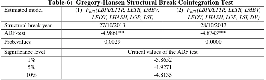
price and its drivers and highlights the great importance to consider structural breaks in the interaction dynamic process of BPI as well as its main determinants(Equation (1), Table-6). These outcomes do not change substantially when accounting for DV (Equation (2), Table-6). The effect of the added dummy variable seems negative and statistically significant as expected (Section-3).

Table-4: The ARDL Bounds Testing Analysis

Dependent variable: DLBPIt

(1) (2)

C 0.6078

(1.0537)

3.4815 (1.1373)

DLBPIt-1 0.11687**

(2.96916)

0.5641** (3.0184)

DLBPIt-2 0.11154**

(2.95493)

0.1557*** (3.8357)

DLBPIt-3 -0.0618

(-1.6440)

-0.0523 (-1.5666)

DLTTRt-1 0.20127***

(9.12259)

0.4846* (1.8352)

DLETRt-1 0.0329*

(1.6778)

0.0825* (1.6934)

DLMBVt-1 0.00134

(0.2775)

0.0049 (0.2057)

DLEOVt-1 0.0030

(0.37838)

0.0428 (1.9022)

DLHASHt-1 0.01192

(0.4814)

0.0075 (0.4132)

DLGPt-1 0.17445

(0.6631)

0.3248 (0.1847)

DLSIt-1 0.1182*

(1.9049)

0.3516* (2.2567)

LBPIt-1 -0.01014

(-1.0310)

0.1602*** (3.2488)

LTTRt-1 0.0038

(0.4752)

0.0336 (1.1308)

LETRt-1 0.0096*

(1.8057)

0.0314 (0.8947)

LMBVt-1 0.0038

(0.6587)

0.0344 (1.2216)

LEOVt-1 0.0034

(0.5983)

0.0137 (0.4755)

LHASHt-1 0.0035*

(1.7380)

0.0092* (1.8607)

LGPt-1 -0.1189

(-1.3637)

-0.0555 (-1.1431)

LSIt-1 0.02128

(0.4324)

-1.0622 (-0.8250)

DV --- -0.0957*

(-1.8796) Diagnostic tests

R-squared SE regression

Breush-Godfrey serial correlation Ramsey Reset test

0.4586 0.8859 0.0955 [0.9089] 0.03503 [0.8516]

0.48 0.7241 0.0133 [0.6214] 0.0217 [0.6528]

(13)

[image:13.595.68.528.79.218.2]

Table -5: The ARDL Bounds Testing Analysis

Estimated model Optimal lag length F-statistic Prob. (1) FBPI (LBPI/LTTR, LETR, LMBV,

LEOV, LHASH, LGP, LSI)

3, 3,4, 1, 0, 0 _4.7029* 0.0106

(2) FBPI (LBPI/LTTR, LETR, LMBV,

LEOV, LHASH, LGP, LSI, DV)

3, 3,4, 1, 0, 0 4.2852* 0.0381

Significance level Critical values

Lower bounds I(0) Upper bounds I(1) 1%

5% 10%

6.84 4.94 4.04

7.84 5.73 4.78

Notes: ***, ** and * imply significance at the 1%, 5% and 10% levels, respectively; Critical values were obtained from Pesaran et al. (2001).

Table-6: Gregory-Hansen Structural Break Cointegration Test

Estimated model (1) FBPI (LBPI/LTTR, LETR, LMBV,

LEOV, LHASH, LGP, LSI)

(2) FBPI (LBPI/LTTR, LETR, LMBV,

LEOV, LHASH, LGP, LSI, DV)

Structural break year 27/10/2013 28/10/2013

ADF-test -4.9861** -4.8743***

Prob.values 0.0029 0.0000

Significance level Critical values of the ADF test 1%

5% 10%

-5.8652 -4.9271 -4.8135 Notes: ***, ** and * imply significance at the 1%, 5% and 10% level, respectively.

[image:13.595.69.535.267.407.2]

(14)

Figure-2: Plots of cumulative sum of recursive and of squares of recursive residuals

(1): FBPI (LBPI/LTTR, LETR, LMBV, LEOV, LHASH, LGP, LSI)

-80 -60 -40 -20 0 20 40 60 80

I II III IV I II III IV

2011 2012

CUSUM 5% Significance

-0.2 0.0 0.2 0.4 0.6 0.8 1.0 1.2

IV I II III IV I II III IV

2011 2012

CUSUM of Squares 5% Significance

(2) : FBPI (LBPI/LTTR, LETR, LMBV, LEOV, LHASH, LGP, LSI, DV)

-80 -60 -40 -20 0 20 40 60 80

2012 2013

CUSUM 5% Significance

-0.2 0.0 0.2 0.4 0.6 0.8 1.0 1.2

2012 2013

CUSUM of Squares 5% Significance

(15)

Figure-3: Plots of cumulative sum of recursive coefficients

(1): FBPI (LBPI/LTTR, LETR, LMBV, LEOV, LHASH, LGP, LGP, LSI)

-400 -300 -200 -100 0 100 200

2011 2012

Recursi ve C(1) Esti mates ± 2 S.E.

-2 0 2 4 6 8

2011 2012

-3 -2 -1 0 1 2 3

2011 2012

-3 -2 -1 0 1 2

2011 2012

-3 -2 -1 0 1

2011 2012

-3 -2 -1 0 1

2011 2012

-.4 -.2 .0 .2 .4 .6

2011 2012

-0.5 0.0 0.5 1.0 1.5 2.0

2011 2012

-6 -4 -2 0 2 4

2011 2012

-20 -10 0 10 20

2011 2012

Recursi ve C(10) Estimates ± 2 S.E.

-30 -20 -10 0 10

2011 2012

-8 -6 -4 -2 0 2

2011 2012

-2 0 2 4 6

2011 2012

-2 0 2 4 6

2011 2012

-.8 -.6 -.4 -.2 .0 .2 .4

2011 2012

-4 -3 -2 -1 0 1

2011 2012

-2 0 2 4 6

2011 2012

-30 -20 -10 0 10 20

2011 2012

-20 0 20 40 60

2011 2012

(2) FBPI (LBPI/LTTR, LETR, LMBV, LEOV, LHASH, LGP, LGP, LSI, DV)

-5 0 5 10 15 20

M4M5 M6 M7 M8 M9 M10M11 M12 2013

-1.2 -0.8 -0.4 0.0 0.4

M4M5 M6 M7 M8 M9 M10M11 M12 2013

-.25 -.20 -.15 -.10 -.05 .00 .05

M4M5 M6 M7 M8 M9 M10M11 M12 2013

-.12 -.08 -.04 .00 .04 .08

M4M5 M6 M7 M8 M9 M10M11M12 2013

-4 -2 0 2 4

M4M5 M6 M7 M8 M9 M10M11M12 2013

-.4 -.2 .0 .2 .4 .6 .8

M4M5 M6 M7 M8 M9 M10M11 M12 2013

-.05 .00 .05 .10

M4M5 M6 M7 M8 M9 M10M11 M12 2013

-.05 .00 .05 .10 .15 .20

M4M5 M6 M7 M8 M9 M10M11 M12 2013

-.2 .0 .2 .4 .6 .8

M4M5 M6 M7 M8 M9 M10M11M12 2013

-0.4 0.0 0.4 0.8 1.2

M4M5 M6 M7 M8 M9 M10M11M12 2013

Recursi ve C(10) E stimates ± 2 S.E.

-6 -4 -2 0 2 4

M4M5 M6 M7 M8 M9 M10M11 M12 2013

-.3 -.2 -.1 .0 .1

M4M5 M6 M7 M8 M9 M10M11 M12 2013

-3 -2 -1 0 1

M4M5 M6 M7 M8 M9 M10M11 M12 2013

-.3 -.2 -.1 .0 .1

M4M5 M6 M7 M8 M9 M10M11M12 2013

-.10 -.05 .00 .05 .10 .15

M4M5 M6 M7 M8 M9 M10M11M12 2013

-.10 -.05 .00 .05 .10

M4M5 M6 M7 M8 M9 M10M11 M12 2013

-.1 .0 .1 .2 .3 .4

M4M5 M6 M7 M8 M9 M10M11 M12 2013

-.3 -.2 -.1 .0 .1

M4M5 M6 M7 M8 M9 M10M11 M12 2013

-1.2 -0.8 -0.4 0.0 0.4 0.8

M4M5 M6 M7 M8 M9 M10M11M12 2013

-.3 -.2 -.1 .0 .1 .2 .3

M4M5 M6 M7 M8 M9 M10M11M12 2013

(16)

From our results reported in Table-7, we clearly notice that Bitcoin price interacts differently with its determinants depending to time periods. In the short-run, the users‟ interest, the exchange-trade ratio, the estimated output volume and the Shangai index affect positively and significantly the BPI. However, the monetary velocity, the hash rate and the gold price have no influence on this digital money. These outcomes change intensely in the long-run, i.e. the speculation, the EOV and the Chinese stock market index which play determinant roles in the short term become without significant influence on Bitcoin price development in the long-run. The impact of ETR on BPI stills positive and significant, but becomes much less important. The effects of MBV and GP on BPI remain insignificant, whereas the hash rate plays a significant role in the long term. Furthermore, the value of ECT

is negative and statistically significant at 5 percent level, which is theoretically correct. It amounts (-7.97E-06), implying that the deviation in the short-run is corrected by 0.0007% towards the long-run equilibrium path. The R-squared value indicates that 44% of Bitcoin price dynamic is explained by the explanatory variables under consideration. These findings change slightly when moving from Equation (1) to Equation (2) that considers the Chinese

Bankruptcy. Both estimates show that investors „attractiveness and the performance of

Chinese market index are the most influent variables on the dynamic of Bitcoin price.

4.2.Innovative accounting approach results

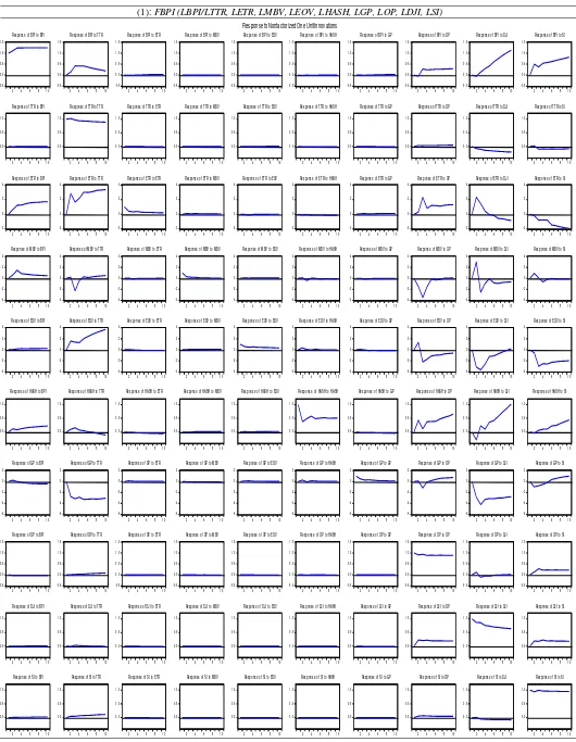
The results of the variance decomposition are reported in Table-8. We find that 69.17% percent of Bitcoin price is explained by its own innovative shocks (Upper Table-8).

The investors‟ attractiveness (TTR) plays the major role in explaining the price dynamic of

Bitcoin (20.34%). The contribution of ETR appears minor, amounting 0.16%. Similarly for Bitcoin monetary velocity, the estimated output volume and the hash rate with respective percentages equal to 0.035%, 0.037% and 0.003%. Gold price explains 0.095% of BPI but we should not forget to mention that the link between GP and BPI appears insignificant in the above results. Additionally, the contribution of Chinese market index (SI) in explaining the Bitcoin dynamic seems sharply intense (10.14%). When considering DV (Lower Table-8), the contributions of speculation and Shangai market index on the evolution of BPI remain dominant.

(17)

responses when accounting for Chinese bankruptcy (Lower graph, Figure-4). The reaction of BPI to TTR and SI still positive, while the contributions of the rest of variables remain very slight or negligible

Table-7: Short-run and long-run Analysis

Dependent variable: LBPIt

(1) (2) Short-run

DLBPIt 0.1252***

(3.1873)

0.3722*** (7.6306)

DLTTRt 0.5269**

(2.8944)

0.3107** (3.2019)

DLETRt 0.1287***

(7.0988)

0.0954*** (5.4125)

DLMBVt 2.7411

(0.2189)

-5.1072 (-1.3082)

DLEOVt 0.0798***

(3.6287)

0.1583*** (3.7943)

DLHASHt 0.0594

(0.5379)

0.3040 (0.1569)

DLGPt -0.2415

(-0.9103)

-0.0238 (-0.9867)

DLSIt 0.3802*

(1.6444)

0.2272** (2.9769)

ECTt -7.97E-06**

(-2.5130)

-3.20E-06* (-1.7186) Long-run

LBPIt 0.1328***

(3.3635)

0.2309*** (4.7347)

LTTRt 0.1434

(0.5414)

0.0279 (1.2933)

LETRt 0.0180*

(1.7073)

0.0222* (1.9182)

LMBVt 0.0043

(0.8892)

0.0287 (0.9623)

LEOVt 0.0073

(0.8993)

-0.0030 (-0.0778)

LHASHt 0.0072*

(1.8478)

0.0076* (1.9784)

LGPt -0.0015

(-0.1556)

0.2140 (0.8852)

LSIt 0.2157

(0.1062)

0.3295 (0.2478)

DV --- -0.0812*

(-1.7697) Diagnostic tests

R-squared SE regression

Breush-Godfrey serial correlation Ramsey Reset test

0.44 0.7812 0.3987 [0.1125] 0.2419 [0.6038]

0.36 0.5376 0.0862 [0.5034] 0.0129 [0.3185]

(18)

Table-8: Variance Decomposition of Bitcoin price

Period S.E. LBPI LTTR LETR LMBV LEOV LHASH LGP LSI

(1) FBPI (LBPI/LTTR, LETR, LMBV, LEOV, LHASH, LGP, LGP, LSI)

1 0.089209 100.0000 0.000000 0.000000 0.000000 0.000000 0.000000 0.000000 0.000000 2 0.133356 69.62125 20.02477 0.099387 0.021195 0.048033 0.000927 0.002721 10.18171 3 0.173881 69.36913 20.14811 0.154151 0.041684 0.040414 0.008345 0.074429 10.16373 4 0.207915 69.31502 20.21095 0.143917 0.034885 0.040420 0.005948 0.079367 10.16948 5 0.237979 69.26216 20.26038 0.154534 0.037175 0.038559 0.004840 0.083554 10.15879 6 0.264822 69.22643 20.29075 0.160299 0.037687 0.038561 0.004506 0.087948 10.15380 7 0.289336 69.20724 20.31188 0.161535 0.037241 0.038131 0.003989 0.091187 10.14878 8 0.311935 69.19196 20.32765 0.163871 0.036489 0.037956 0.003689 0.093026 10.14535 9 0.333019 69.18027 20.33966 0.165645 0.035905 0.037888 0.003476 0.094519 10.14264 10 0.352847 69.17171 20.34903 0.166578 0.035233 0.037921 0.003293 0.095698 10.14054

(2) FBPI (LBPI/LTTR, LETR, LMBV, LEOV, LHASH, LGP, LGP, LSI, DV)

(19)

Figure-4: Impulse Response Functio

(1): FBPI (LBPI/LTTR, LETR, LMBV, LEOV, LHASH, LGP, LSI)

-0.5 0.0 0.5 1.0 1.5

2 4 6 8 10

Response of BP I to B P I

-0.5 0.0 0.5 1.0 1.5

2 4 6 8 10

Response of BP I to TTR

-0.5 0.0 0.5 1.0 1.5

2 4 6 8 10

Response of B P I to E TR

-0.5 0.0 0.5 1.0 1.5

2 4 6 8 10

Response of B P I to MB V

-0.5 0.0 0.5 1.0 1.5

2 4 6 8 10

Response of B P I to EOV

-0.5 0.0 0.5 1.0 1.5

2 4 6 8 10

Response of B P I to HA S H

-0.5 0.0 0.5 1.0 1.5

2 4 6 8 10

Response of BP I to GP

-0.5 0.0 0.5 1.0 1.5

2 4 6 8 10

Response of B PI to S I

0.0 0.5 1.0

2 4 6 8 10

Response of TTR to BP I

0.0 0.5 1.0

2 4 6 8 10

Response of TTR to TTR

0.0 0.5 1.0

2 4 6 8 10

Response of TTR to E TR

0.0 0.5 1.0

2 4 6 8 10

Response of TTR to MB V

0.0 0.5 1.0

2 4 6 8 10

Response of TTR to EOV

0.0 0.5 1.0

2 4 6 8 10

Response of TTR to HA S H

0.0 0.5 1.0

2 4 6 8 10

Response of TTR to GP

0.0 0.5 1.0

2 4 6 8 10

Response of TTR to S I

-2 0 2 4

2 4 6 8 10

Response of E TR to BP I

-2 0 2 4

2 4 6 8 10

Response of ETR to TTR

-2 0 2 4

2 4 6 8 10

Response of E TR to E TR

-2 0 2 4

2 4 6 8 10

Response of E TR to MB V

-2 0 2 4

2 4 6 8 10

Response of E TR to EOV

-2 0 2 4

2 4 6 8 10

Response of E TR to HA S H

-2 0 2 4

2 4 6 8 10

Response of E TR to GP

-2 0 2 4

2 4 6 8 10

Response of E TR to S I

-4 -2 0 2

2 4 6 8 10

Response of MB V to B P I

-4 -2 0 2

2 4 6 8 10

Response of MB V to TTR

-4 -2 0 2

2 4 6 8 10

Response of MB V to E TR

-4 -2 0 2

2 4 6 8 10

Response of MB V to MB V

-4 -2 0 2

2 4 6 8 10

Response of MB V to E OV

-4 -2 0 2

2 4 6 8 10

Response of MB V to HA S H

-4 -2 0 2

2 4 6 8 10

Response of MB V to GP

-4 -2 0 2

2 4 6 8 10

Response of MB V to S I

-4 -2 0 2

2 4 6 8 10

Response of E OV to B P I

-4 -2 0 2

2 4 6 8 10

Response of EOV to TTR

-4 -2 0 2

2 4 6 8 10

Response of E OV to E TR

-4 -2 0 2

2 4 6 8 10

Response of E OV to MB V

-4 -2 0 2

2 4 6 8 10

Response of EOV to E OV

-4 -2 0 2

2 4 6 8 10

Response of E OV to HA S H

-4 -2 0 2

2 4 6 8 10

Response of E OV to GP

-4 -2 0 2

2 4 6 8 10

Response of E OV to S I

0.0 0.5 1.0

2 4 6 8 10

Response of HA S H to BP I

0.0 0.5 1.0

2 4 6 8 10

Response of HA S H to TTR

0.0 0.5 1.0

2 4 6 8 10

Response of HA S H to ETR

0.0 0.5 1.0

2 4 6 8 10

Response of HA S H to MB V

0.0 0.5 1.0

2 4 6 8 10

Response of HA S H to EOV

0.0 0.5 1.0

2 4 6 8 10

Response of HA S H to HA S H

0.0 0.5 1.0

2 4 6 8 10

Response of HA S H to GP

0.0 0.5 1.0

2 4 6 8 10

Response of HA S H to SI

-4 -2 0 2

2 4 6 8 10

Response of GP to B P I

-4 -2 0 2

2 4 6 8 10

Response of GP to TTR

-4 -2 0 2

2 4 6 8 10

Response of GP to E TR

-4 -2 0 2

2 4 6 8 10

Response of GP to MB V

-4 -2 0 2

2 4 6 8 10

Response of GP to EOV

-4 -2 0 2

2 4 6 8 10

Response of GP to HA S H

-4 -2 0 2

2 4 6 8 10

Response of GP to GP

-4 -2 0 2

2 4 6 8 10

Response of GP to S I

0.0 0.5 1.0

2 4 6 8 10

Response of SI to B P I

0.0 0.5 1.0

2 4 6 8 10

Response of SI to TTR

0.0 0.5 1.0

2 4 6 8 10

Response of SI to E TR

0.0 0.5 1.0

2 4 6 8 10

Response of S I to MB V

0.0 0.5 1.0

2 4 6 8 10

Response of SI to EOV

0.0 0.5 1.0

2 4 6 8 10

Response of S I to HA S H

0.0 0.5 1.0

2 4 6 8 10

Response of SI to GP

0.0 0.5 1.0

2 4 6 8 10

Response of SI to S I

Response to Nonfactorized One Unit Innovations

(2): FBPI (LBPI/LTTR, LETR, LMBV, LEOV, LHASH, LGP, LSI, DV)

-.2 .0 .2 .4 .6

2 4 6 8 10 Response of B P I to B P I

-.2 .0 .2 .4 .6

2 4 6 8 10 Response of B P I to TTR

-.2 .0 .2 .4 .6

2 4 6 8 10 Response of B P I to E TR

-.2 .0 .2 .4 .6

2 4 6 8 10 Response of B P I to MB V

-.2 .0 .2 .4 .6

2 4 6 8 10 Response of B P I to E OV

-.2 .0 .2 .4 .6

2 4 6 8 10 Response of B P I to HA S H

-.2 .0 .2 .4 .6

2 4 6 8 10 Response of B P I to GP

-.2 .0 .2 .4 .6

2 4 6 8 10 Response of B P I to S I

-.4 .0 .4 .8

2 4 6 8 10 Response of TTR to B P I

-.4 .0 .4 .8

2 4 6 8 10 Response of TTR to TTR

-.4 .0 .4 .8

2 4 6 8 10 Response of TTR to E TR

-.4 .0 .4 .8

2 4 6 8 10 Response of TTR to MB V

-.4 .0 .4 .8

2 4 6 8 10 Response of TTR to E OV

-.4 .0 .4 .8

2 4 6 8 10 Response of TTR to HA S H

-.4 .0 .4 .8

2 4 6 8 10 Response of TTR to GP

-.4 .0 .4 .8

2 4 6 8 10 Response of TTR to S I

-.01 .00 .01

2 4 6 8 10 Response of E TR to B P I

-.01 .00 .01

2 4 6 8 10 Response of E TR to TTR

-.01 .00 .01

2 4 6 8 10 Response of E TR to E TR

-.01 .00 .01

2 4 6 8 10 Response of E TR to MB V

-.01 .00 .01

2 4 6 8 10 Response of E TR to E OV

-.01 .00 .01

2 4 6 8 10 Response of E TR to HA S H

-.01 .00 .01

2 4 6 8 10 Response of E TR to GP

-.01 .00 .01

2 4 6 8 10 Response of E TR to S I

-0.5 0.0 0.5 1.0

2 4 6 8 10 Response of MB V to B P I

-0.5 0.0 0.5 1.0

2 4 6 8 10 Response of MB V to TTR

-0.5 0.0 0.5 1.0

2 4 6 8 10 Response of MB V to E TR

-0.5 0.0 0.5 1.0

2 4 6 8 10 Response of MB V to MB V

-0.5 0.0 0.5 1.0

2 4 6 8 10 Response of MB V to E OV

-0.5 0.0 0.5 1.0

2 4 6 8 10 Response of MB V to HA S H

-0.5 0.0 0.5 1.0

2 4 6 8 10 Response of MB V to GP

-0.5 0.0 0.5 1.0

2 4 6 8 10 Response of MB V to S I

-.2 .0 .2 .4 .6

2 4 6 8 10 Response of E OV to B P I

-.2 .0 .2 .4 .6

2 4 6 8 10 Response of E OV to TTR

-.2 .0 .2 .4 .6

2 4 6 8 10 Response of E OV to E TR

-.2 .0 .2 .4 .6

2 4 6 8 10 Response of E OV to MB V

-.2 .0 .2 .4 .6

2 4 6 8 10 Response of E OV to E OV

-.2 .0 .2 .4 .6

2 4 6 8 10 Response of E OV to HA S H

-.2 .0 .2 .4 .6

2 4 6 8 10 Response of E OV to GP

-.2 .0 .2 .4 .6

2 4 6 8 10 Response of E OV to S I

-.08 -.04 .00 .04 .08 .12

2 4 6 8 10 Response of HA S H to B P I

-.08 -.04 .00 .04 .08 .12

2 4 6 8 10 Response of HA S H to TTR

-.08 -.04 .00 .04 .08 .12

2 4 6 8 10 Response of HA S H to E TR

-.08 -.04 .00 .04 .08 .12

2 4 6 8 10 Response of HA S H to MB V

-.08 -.04 .00 .04 .08 .12

2 4 6 8 10 Response of HA S H to E OV

-.08 -.04 .00 .04 .08 .12

2 4 6 8 10 Response of HA S H to HA S H

-.08 -.04 .00 .04 .08 .12

2 4 6 8 10 Response of HA S H to GP

-.08 -.04 .00 .04 .08 .12

2 4 6 8 10 Response of HA S H to S I

-.005 .000 .005 .010 .015

2 4 6 8 10 Response of GP to B P I

-.005 .000 .005 .010 .015

2 4 6 8 10 Response of GP to TTR

-.005 .000 .005 .010 .015

2 4 6 8 10 Response of GP to E TR

-.005 .000 .005 .010 .015

2 4 6 8 10 Response of GP to MB V

-.005 .000 .005 .010 .015

2 4 6 8 10 Response of GP to E OV

-.005 .000 .005 .010 .015

2 4 6 8 10 Response of GP to HA S H

-.005 .000 .005 .010 .015

2 4 6 8 10 Response of GP to GP

-.005 .000 .005 .010 .015

2 4 6 8 10 Response of GP to S I

-0.5 0.0 0.5 1.0

2 4 6 8 10 Response of S I to B P I

-0.5 0.0 0.5 1.0

2 4 6 8 10 Response of S I to TTR

-0.5 0.0 0.5 1.0

2 4 6 8 10 Response of S I to E TR

-0.5 0.0 0.5 1.0

2 4 6 8 10 Response of S I to MB V

-0.5 0.0 0.5 1.0

2 4 6 8 10 Response of S I to E OV

-0.5 0.0 0.5 1.0

2 4 6 8 10 Response of S I to HA S H

-0.5 0.0 0.5 1.0

2 4 6 8 10 Response of S I to GP

-0.5 0.0 0.5 1.0

2 4 6 8 10 Response of S I to S I

(20)

Furthermore, we evaluate whether there is a causal relationship between the explanatory variables in question and the Bitcoin price dynamic. Before testing the non-causality hypothesis, we start by examining the residuals using the LM test for serial independence against the alternative of AR(k)/MA(k), for k = 1, ...., 12. From the findings reported in Table-9, the serial correlation may be removed at the maximum lag length which is 3. The non-causality test findings are reported in Table-10. It is clearly notable that we can reject the null hypothesis of no causality DLTTR to DLBPI, from DLETR to DLBPI and from

DLSI to DLBPI, while the reverse link is not supported confirming therefore the above outcomes obtained through the ARDL Bounds Testing method and the innovation accounting approach (variance decomposition and impulse responses). For the rest of variables, we accept the null hypothesis of non-causality (except for the relationship that runs from DLBPI

to DLHASH and the link running from DLBPI to DLMBV). These results may very useful for businesses, investors and regulators.

Table-9: VEC Residual Serial Correlation LM Tests

Null Hypothesis: no serial correlation at lag order h

Lags LM-Stat Prob

1 165.7815 0.0000

2 162.7223 0.0000

3 172.6073 0.0000

4 74.87208 0.1661

5 108.8017 0.0004

6 52.65505 0.8435

7 86.67175 0.0312

8 59.58174 0.6333

9 73.80962 0.1882

10 67.46570 0.3595

11 69.17378 0.3071

12 88.51908 0.0229

Table-10: VEC Granger Causality/Block Exogeneity Wald Tests

Dependent variable: DLBPI

Excluded Chi-sq df Prob

DLTTR≠DLBPI

DLBPI≠DLTTR

4.4897 0.7034

2 2

0.0474 0.7035

DLETR≠DLBPI

DLBPI≠DLETR

2.9722 4.2470

2 2

0.0226 0.1196

DLMBV≠DLBPI DLBPI≠DLMBV

0.9299 13.698

2 2

0.6281 0.0011

DLEOV≠DLBPI DLBPI≠DLEOV

1.1004 1.9394

2 2

0.5768 0.3792

DLHASH≠DLBPI DLBPI≠DLHASH

0.3544 6.2336

2 2

0.8376 0.0443

DLGP≠DLBPI

DLBPI≠DLGP

1.0579 1.0588

2 2

0.3574 0.3572

DLSI≠DLBPI DLBPI≠DLSI

3.5051 1.4394

2 2

(21)

5. Robustness

The above findings clearly indicate that the investors attractiveness, the exchange-trade ratio, the estimated output volume and the Shangai index affect positively and significantly the Bitcoin price, while the monetary velocity, the hash rate and the gold price have no influence in the short term. However, the speculative nature of Bitcoin, the EOV and the Chinese stock market index which play the major role in the short-run appear without statistically significant impact on Bitcoin price in the long-run. The influence of ETR on BPI

becomes less strong, whereas the effects of MBV and GP on BPI remain statistically insignificant in the majority of cases. The hash rate plays a significant role on explaining the dynamic of this nascent virtual currency. To check properly and appropriately the robustness of these evidences, we re-estimate the relationships between Bitcoin price and its determinants by incorporating a dummy variable relative to the bankruptcy of Chinese trading company, using the same methods (i.e. an ARDL Bounds Testing method, an innovation accounting approach by simulating variance decomposition and impulse response function and VEC Granger causality test). Comparing these results with those of Equation without dummy variable, we put in evidence that the effects of TTR, ETR, MBV, EOV, HASH, GP and

SI are solid and unambiguous. Beyond the nuances of short and long terms, the present study confirms the speculative nature of Bitcoin without neglecting its usefulness in economic reasons and the importance of accounting for Chinese stock market and the processing power of Bitcoin network. At this stage, we can consider it only as a risky investment, short-term hedge and partially as business income. Nonetheless, this new crypto-currency seems far from being a safe haven and a long-term promise.

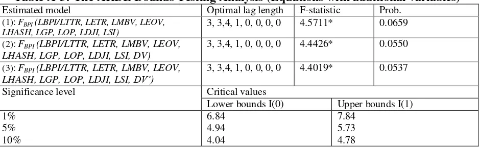
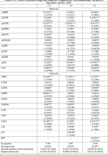
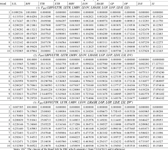
To be more effective, we believe that the use of other combinations of variables by adding other variables in Equations 3 and 4 (oil price4, Dow Jones index5 and a dummy variable denoting the closing of road silk by FBI6) that may affect the Bitcoin price based on few studies on the field (Ciaian et al. 2014, for example) may be fruitful. Nevertheless, the obtained findings reveal that the effects of the additional time series are in the majority of cases insignificant and more importantly the estimates become sharply unstable (see Figure A-1, particularly). More details about outcomes are summarized in Table A-1, Table A-2, Table A-3, Table A-4, Table A-5, Table A-6, Figure A-2 and Figure A-3.

4

Palombizio and Morris (2012) find that oil price (OP) is a potential factor that may affect intensely the inflation outcomes. If the price of oil indicates great ups and downs (i.e. sizeable volatility), the Bitcoin depreciates. Besides, the exchange rate may reflect inflationary pressures affecting positively the prices of this crypto-currency.

5

The relationship between Bitcoin price and the Dow Jones index (DJI) appears complex, since the two variables seem sometimes correlated but not usually. After the announcement of American satellite TV provider that it would start accepting Bitcoin as payment tool, the prices of this digital money increased approximately by $40 touching the level of $ 600, while the Dow Jones Index was down by 300 points. A perfect example of how the Bitcoin and the American markets have been initially unrelated. Nevertheless, the offshoots of Al-Qaeda over different cities in Iraq and the Obama‟s declaration (i.e. America will not send the military in order to fight off the terrorist organizations) have affected Bitcoin price and simultaneously Dow Jones index. Due to the sizeable connection between the turmoil and Bitcoin‟s value, the price of Bitcoin started dropping and as response the Dow Jones index started falling by 200 points. This implies that there is some connection between both variables. For details, you can refer to: http://coinbrief.net/bitcoin-price-news-analysis/

6

(22)

6.

Concluding remarks and Policy implications

The present research attempts to reach clearer knowledge about the nascent crypto-currency (Bitcoin) by effectively answering the following questions: What Bitcoin looks like? Is it a safe haven or a “speculative bubble”? Is it a business income, a short-term hedge, a risky investment or a long-term promise?

To this end, we have regressed Bitcoin price on investors‟ attractiveness, exchange-trade volume, monetary Bitcoin velocity, estimated output volume, hash rate, gold price and Shangai market index using an ARDL Bounds Testing method, an innovation accounting approach and VEC Granger causality test for daily data covering the period from December 2010 to June 2014. By doing so, we have checked the speculative nature of Bitcoin. We also provide insightful evidence that Bitcoin may be used for economic reasons but there is any sign of being a safe haven. By accounting for the Chinese trading bankruptcy, the contribution of the speculative behavior of investors and the performance of Chinese stock market remain dominant, while the role of Bitcoin as transactions tool dissipates in the long-run, highlighting the robustness of our results. Intuitively, by using other combinations of variables by adding other time series (including oil price, Dow Jones index and a dummy variable denoting the closing of road silk by FBI) to confirm our findings, the estimates become remarkably unstable. It is important to mention here that these last variables have no statistically significant influence in the majority of cases in Bitcoin price development.

In a nutshell, Bitcoin behaves heavily as a “speculative bubble”, short-term hedge and risky investment and partially as business income. This new digital money is far from being a long-term promise, especially when considering that this virtual currency faces a great challenge (in particular a structural economic problem) regarding its limited amount recording 21 million units in 2140, implying that the money supply would not expand after this date. If this digital currency succeeds really to displace fiat currencies, it would exert great deflationary pressures.

This goes without saying that these findings should be treated with caution. Nobody is, up to now, able to estimate the true value of Bitcoin. The fact that the dynamic of the focal digital money is uncertain even more sustains speculation. Without tackling the main causes, the virtual currency seems highly correlated to the speculative behaviors of investors and people who hold this money. Bitcoin is not issued by banking system and even less by governments, but by a computing algorithm. Unfortunately, the majority of Bitcoin users have not heavily acknowledged about mathematical programs, and it is of course unknown for them how far it can go. The volatility of Bitcoin and the difficulty of processing power network are likely to discourage investors and users of this money. Intuitively, China represents the most active Bitcoin market in the world. The sizeable attention to this crypto-currency in the Chinese media has drawn a huge number of investors. However, the attitude of Chinese practitioners, advisers and regulators towards Bitcoin is ambiguous, yielding to much more speculation. This may reinforce the evidence thereby Bitcoin is short-term hedge, a risky investment. We cannot confirm if this currency may be considered as long-term

promise since the contribution of investors‟ interest appears dominant among the different

estimations. This may support the conclusion of Bouoiyour et al. (2014) showing that it is

(23)

(24)

References

Aguiar-Conraria, L. and Soares, M-J. (2011), “The continuous wavelet transform: A

primer.” NIPE working paper n°16, University of Minho.

Bouoiyour, J., Selmi, R. and Tiwari, A-K. (2014), “Is Bitcoin Business Income or Speculative Bubble? Unconditional vs. Conditional Frequency Domain Analysis.” Working paper, CATT, University of Pau.

Breitung, J., and Candelon, B. (2006), “Testing for short and long-run causality: a

frequency domain approach.” Journal of Econometrics, 132, 363-378.

Buchholz, M., Delaney, J., Warren, J. and Parker, J. (2012), “Bits and Bets, Information, Price Volatility, and Demand for Bitcoin.” Economics 312, http://www.bitcointrading.com/pdf/bitsandbets.pdf

Ciaian, P., Rajcaniova, M. and Kancs, D. (2014), “The Economics of BitCoin Price

Formation”. http://arxiv.org/ftp/arxiv/papers/1405/1405.4498.pdf

Glaster, F., Kai, Z., Haferkorn, M., Weber, M. and Sieiring, M. (2014), “Bitcoin -

asset or currency? Revealing users‟hidden intentions.” Twenty Second European Conference

on Information Systems. http://ecis2014.eu/E-poster/files/0917-file1.pdf

Gregory, A.W. and Hansen, B.E. (1996), “Residual based Tests for Co-integration in Models with Regime Shifts.” Journal of Econometrics, 70, 99-126.

Kristoufek, L. (2013), “BitCoin meets Google Trends and Wikipedia: Quantifying the

relationship between phenomena of the Internet era.” Scientific Reports 3 (3415), 1-7.

Kristoufek, L. (2014), “What are the main drivers of the Bitcoin price? Evidence from

wavelet coherence analysis.” http://arxiv.org/pdf/1406.0268.pdf

Glouderman, L. (2014), “Bitcoin‟s Uncertain Future in China.” USCC Economic Issue Brief n° 4, May 12.

Ng, E.K. and Chan, J.C. (2012), “Geophysical Applications of Partial Wavelet Coherence and Multiple Wavelet Coherence.” American Meteological Society, December.

DOI: 10.1175/JTECH-D-12-00056.1

Palombizio E. and Morris, I. (2012), “Forecasting Exchange Rates using Leading

Economic Indicators.” Open Access Scientific Reports 1(8), 1-6.

Pesaran, M. and Shin, Y. (1999), “An Autoregressive Distributed Lag Modeling

Approach to Cointegration Analysis.” S. Strom, (ed) Econometrics and Economic Theory in the 20th Century, Cambridge University.

Pesaran, M.H., Y. Shin., and Smith R. (2001), “Bounds testing approaches to the

analysis of level relationships.” Journal of Applied Econometrics, 16, 289-326.

Piskorec, P., Antulov-Fantulin, N., Novak, P.K., Mozetic, I., Grcar, M., Vodenska, I.

and Šmuc, T. (2014), “News Cohesiveness: an Indicator of Systemic Risk in Financial

Markets.” arXiv:1402.3483v1 [cs.SI], http://arxiv.org/pdf/1402.3483v1.pdf

Yermack, D. (2013), “Is Bitcoin a Real Currency? An economic appraisal.” NBER

(25)

Appendices

Table-A.1: Lag-order selection (Equations with additional variables)

Lag LogL LR FPE AIC SC HQ

(1) : FBPI(LBPI/LTTR, LETR, LMBV, LEOV, LHASH, LGP, LOP, LDJI, LSI)

0 3678.627 NA* 2.36e-06* -10.11759* -10.04801* -10.09074* 1 3678.644 0.032814 2.37e-06 -10.11488 -10.03897 -10.08558 2 3678.673 0.057395 2.38e-06 -10.11220 -10.02997 -10.08046 3 3678.675 0.003638 2.38e-06 -10.10945 -10.02089 -10.07527

(2) : FBPI(LBPI/LTTR, LETR, LMBV, LEOV, LHASH, LGP, LOP, LDJI, LSI, DV)

0 782.4109 NA 0.006972 -2.128030 -2.058447 -2.101176 1 788.0603 11.11191 0.006883 -2.140856 -2.064947* -2.111560* 2 791.0228 5.818642 0.006846 -2.146270* -2.064035 -2.114533 3 792.0847 2.082820 0.006844* -2.146441 -2.05738 -2.112262

(3) : FBPI(LBPI/LTTR, LETR, LMBV, LEOV, LHASH, LGP, LOP, LDJI, LSI, DV’)