Linear Inferential Modeling: Theoretical Perspectives, Extensions, and Comparative Analysis

http://dx.doi.org/10.4236/ica.2012.34042 Published Online November 2012 (http://www.SciRP.org/journal/ica)

Linear Inferential Modeling: Theoretical Perspectives,

Extensions, and Comparative Analysis

Muddu Madakyaru1, Mohamed N. Nounou1*, Hazem N. Nounou2 1

Chemical Engineering Program, Texas A & M University, Doha, Qatar 2

Electrical and Computer Engineering Program, Texas A & M University, Doha, Qatar Email: *[email protected]

Received July 26,2012; revised August 26, 2012; accepted September 4, 2012

ABSTRACT

Inferential models are widely used in the chemical industry to infer key process variables, which are challenging or ex- pensive to measure, from other more easily measured variables. The aim of this paper is three-fold: to present a theo- retical review of some of the well known linear inferential modeling techniques, to enhance the predictive ability of the regularized canonical correlation analysis (RCCA) method, and finally to compare the performances of these techniques and highlight some of the practical issues that can affect their predictive abilities. The inferential modeling techniques considered in this study include full rank modeling techniques, such as ordinary least square (OLS) regression and ridge regression (RR), and latent variable regression (LVR) techniques, such as principal component regression (PCR), partial least squares (PLS) regression, and regularized canonical correlation analysis (RCCA). The theoretical analysis shows that the loading vectors used in LVR modeling can be computed by solving eigenvalue problems. Also, for the RCCA method, we show that by optimizing the regularization parameter, an improvement in prediction accuracy can be achieved over other modeling techniques. To illustrate the performances of all inferential modeling techniques, a com- parative analysis was performed through two simulated examples, one using synthetic data and the other using simu- lated distillation column data. All techniques are optimized and compared by computing the cross validation mean square error using unseen testing data. The results of this comparative analysis show that scaling the data helps improve the performances of all modeling techniques, and that the LVR techniques outperform the full rank ones. One reason for this advantage is that the LVR techniques improve the conditioning of the model by discarding the latent variables (or principal components) with small eigenvalues, which also reduce the effect of the noise on the model prediction. The results also show that PCR and PLS have comparable performances, and that RCCA can provide an advantage by opti- mizing its regularization parameter.

Keywords: Inferential Modeling; Latent Variable Regression; Regularized Canonical Correlation Analysis; Distillation

Columns

1. Introduction

Models play an important role in various process opera- tions, such as process control, monitoring, and optimiza- tion. In process control, where measuring the controlled variable (s) is difficult, it is usually relied on inferential models that can estimate the controlled variable (s) from other more easily measured variables. For example, the control of distillation column compositions requires the availability of inferential models that can accurately pre- dict the compositions from other variables, such as tem- perature and pressure at different trays of the column. These inferential models are expected to provide accurate predictions of the output variables over a wide range of operating conditions. However, constructing such infer-

ential models is usually associated with many challenges, which include accounting for the presence of measure- ment noise in the data and dealing with collinearity or redundancy among the variables.

the conditioning of the input covariance matrix [5-7], and include Ridge Regression (RR). RR reduces the varia- tions in the model parameters by imposing a penalty on the L2 norm of their estimated values. RR also has a

Bayesian interpretation, where the estimated model pa- rameters are obtained by maximizing a posterior density in which the prior density function is a zero mean Gaus- sian distribution [8].

Latent variable regression (LVR) models, on the other hand, deal with collinearity by transforming the variables so that most of the data information is captured in a smaller number of variables that are used to construct the model. In other words, LVR models perform regression on a small number of latent variables that are linear com- binations of the original variables. This generally results in well-conditioned models and good predictions [9]. LVR model estimation techniques include principal com- ponent regression (PCR) [5,10], partial least squares (PLS) [5,11,12], and regularized canonical correlation analysis (RCCA) [13-16]. PCR is performed in two main step: transform the input variables using principal com- ponent analysis (PCA), and then construct a simple model relating the input to the transformed inputs (prin- cipal components) using ordinary least squares (OLS). Thus, PCR completely ignores the output(s) when de- termining the principal components. Partial least squares (PLS), on the other hand, transforms the variables taking the input-output relationship into account by maximizing the covariance between the transformed inputs and out- puts variables. Therefore, PLS has been widely used in practice, such as in the chemical industry to estimate distillation column compositions [1,17-19]. Other LVR model estimation methods include regularized canonical correlation analysis (RCCA). RCCA is an extension of another estimation technique called canonical correlation analysis (CCA), which determines the transformed input variables by maximizing the correlation between the transformed inputs and the output(s) [13,20]. Thus, CCA also takes the input-output relationship into account when transforming the variables. CCA, however, re- quires computing the inverses of the input covariance matrix. Thus, in the case of collinearity among the vari- ables, regularization of these matrices is performed to enhance the conditioning of the estimated model, which is referred to as regularized CCA (RCCA). Since the covariance and correlation of the transformed variables are related, RCCA reduces to PLS under a certain as- sumptions.

There are three main objectives in this paper. The first objective is to theoretically review the formulations and the underlying assumptions of some of the inferential model estimation techniques, which include OLS, RR, PCR, PLS, and RCCA. This theoretical review will shed some light on the similarities and differences among

these modeling techniques. The second objective is to enhance the prediction ability of LVR inferential models by optimizing the regularization parameter of the RCCA modeling method. The third objective of this paper is to compare the performances of these techniques through two simulated examples, one using synthetic data and the other using simulated distillation column data. This comparative antilysis also provides some insight about some of the practical issues involved in constructing in- ferential models.

The remainder of this paper is organized as follows. In Section 2, a problem statement is presented followed by a theoretical review of the various inferential model es- timation techniques in Section 3. This theoretical discus- sion includes full rank models (such as OLS and RR) and latent variable regression models (such as PCR, PLS, ad RCCA). This discussion presented an extension to opti- mize the RCCA to enhance its prediction ability. Then, in Section 4, the various modeling techniques are compared through two simulated examples, one involving synthetic data and the other involving distillation column data. Finally, some concluding remarks are presented in Sec- tion 5.

2. Problem Statement

This work addresses the problem of developing linear inferential models that can be used to estimate or infer key process variables that are not easily measured from other more easily measured variables. All variables, in- puts and outputs, are assumed to be contaminated with additive zeros mean Gaussian noise. Also, it is assumed that there exists a strong collinearity among the variables. Thus, given measurements of the input and output data, it is desired to construct a linear model of the form,

,

 

y Xb ε n m

(1)

where,   n1

is the input matrix, 

X y

1

m is the

output vector, b 

1

n is the unknown model parame-

ter vector, and ε  is the model error, respectively. Several estimation techniques have been developed to solve this modeling problem; some of the full rank mod-els and latent variable regression modmod-els are described in the following section. In this paper, however, we seek to review the formulations of these inferential modeling methods, present an extension of the RCCA method for enhanced prediction, and provide some insight about the performances of these techniques along with a discission of some of the practical aspects involved in inferential modeling.

3. Theoretical Formulations of Linear

Inferential Models

full rank and latent variable regression model estimation techniques is presented. Full rank modeling techniques include ordinary least square (OLS) regression and ridge regression (RR); while latent variable regression tech- niques include principal component regression (PCR), partial least squares (PLS), and regularized canonical correlation analysis (RCCA). The objective behind this theoretical presentation of the various inferential model- ing techniques is to provide some insight about the simi- larities and differences between these techniques through their formulations and the assumptions made by each technique.

3.1. Full Rank Models

3.1.1. Ordinary Least Squares (OLS)

Ordinary least square regression is one of the most popular model estimation techniques, in which the model parameters are estimated by minimizing the L2 norm of

the residual error or the sum of residual square error [5,10]. Therefore, the model parameter vector is esti- mated by solving the following optimization problem:



2



2

,Xby

ˆ

b





1

.

T T

ˆ_{arg min}

b

b (2)

which has the following closed form solution for the pa- rameter vector :

ˆ _{X X}  _{X y}



T





b (3)

Note that the OLS solution (3) requires inverting the matrix X X . Therefore, when



X XT



ˆ

b

is close to singularity (due to collinearity among the input variables), the variance of estimated parameter vector increases, which also increases the uncertainty about its estimation. One way to deal with this collinearity problem is through regularization of the estimated parameters as performed in ridge regression (RR), which is described next.

3.1.2. Ridge Regression (RR)

To reduce the uncertainty about the estimated model pa- rameters, RR not only minimizes the L2 norm of the

model prediction error (as in OLS), but also the L2 norm

of the estimated parameters themselves [6]. Thus, RR can be formulated as follows:



2 2



2 2

, b



1

,

T T

ˆ_{arg min X y}

b

b b ₍₄₎

which has the following closed form solution:



ˆ _{X X I}  _{X y}

m m

 

b (5)

where λis a positive constant, and I  is the iden- tity matrix. It can be seen from Equation (5) that adding

λI to the matrix X XT before inverting improves the conditioning of the estimation problem. The L2 regulari-

zation of the model parameters in RR makes it an effec- tive means to achieve numerical stability in finding the solution and also to improve the predictive performance of the estimated inferential model.

3.2. Latent Variable Regression (LVR) Models

Dealing with the large number of highly correlated mea- sured variables involved in inferential models is one of the key issues that affect their estimation and predictive abilities. It is known that over-parameterized models can fit the original data well, but they usually lead to poor predictions. Multivariate statistical projection methods such as PCR, PLS, and RCCA can be utilized to deal with this issue by performing regression on a smaller number of transformed variables, called latent variables (or principal components), which are linear combinations of the original variables. This approach, which is called latent variable regression (LVR), generally results in well-conditioned parameter estimates and good model predictions [9]. In the subsequent section, the problem formulations and solution techniques for PCR, PLS, and RCCA are presented.

However, before we introduce these methods, let’s in- troduce some definitions. Let the matrix D be defined as the augmented scaled input and output data, i.e.,





D X y . Note that scaling the data is performed by making each variable (input and output) zero mean with a unit variance. Then, the covariance of D can be defined as follows [16]:







 









 





  

T

T

T T

T T

E

E

E E

E E





 

 



 

 

 

  

 

 

XX Xy

yX yy

C DD

X y X y

X X X y y X y y C C

C C

(6)

where the matrices CXX, CXy, CyX and Cyy are of

dimensions



m m



,



m1



,



m1



, and

 

1 1 , respectively.

Since the latent variable model will be developed us-ing transformed variables, let’s define the transformed inputs as follows:

z_iXa_i, (7) where zi is the i latent input variable ,

and i is the input loading vector, which is of

di-mension

th





1, ,

i  m

a _ith



m1



.

3.2.1. Principal Component Regression (PCR)

reducing their dimension using principal component analysis (PCA), which utilizes singular value decomposi- tion (SVD) to compute the latent variables or principal components. Then, it constructs a simple linear model between the latent variables and the output using ordi- nary least square (OLS) regression [5,10]. Therefore, PCR can be formulated as two consecutive estimation problems. First, the loading vectors are estimated by maximizing the variance of the estimated principal com- ponents as follows:

 

ˆ argmax var

. . 1;

i

i i

T

i i i

s t  

a

a z

a a z X





1, , i i m    a (8)

which, since the data are mean centered, can also be ex- pressed in terms of the input covariance matrix CXX



1, ,



i i  m

C a

ˆ_{i i} ,ˆ_i

as follows:

ˆ argmax

. . 1.

T i i i T i i s t   XX a a a a a (9)

The solution of the optimization problem (9) can be obtained using the method of Lagrangian multiplier, which results in the following eigenvalue problem (see proof in Appendix A):





XX

C a a (10) which means that the estimated loading vectors are the eigenvectors of the matrix XX

Secondly, after the principal components (PCs) are es- timated, a subset (or all) of these PCs (which correspond to the largest eigenvalues) are used to construct a simple linear model, that relates these PCs to the output, using OLS. Let the subset of PCs used to construct the model be defined as 1

C .

p  

Z _zz _, where p m , then the model relating these PCs to the output can be estimated as follows:



2



2

n

ˆ _{arg mi y}

 

 Zβ

 

_T 1 _T

(11)

which has the following solution,

ˆ _{Z Z}  _{Z y.}

p m 

β (12)

Note that if all the estimated principal components are used in constructing the inferential model (i.e.,

3.2.2. Partial Least Square (PLS)

PLS computes the input loading vectors, i, by maxi-

mizing the covariance between the estimated latent vari- able

a

ˆ_i

z and model output, y, i.e., [20,21]:





ˆ argmaxcov ,

. . 1;

i

i i

T

i i i i

s t



 

a

a z y

a a z Xa

1, , ,

i p p m

(13)



 . Since zi i

where,  Xa and the data

are mean centered, equation (13) can also be expressed in terms of the covariance matrix CXy

ˆ argmax

. . 1.

i T i i T i i s t   as follows: Xy a

a a C

a a

2

ˆ_{i i} ˆ_i

(14)

The solution of the optimization problem 14 can be obtained using the method of Lagrangian multiplier, which leads to the following eigenvalue problem (see proof in Appendix B):

 ), then PCR reduces to OLS. Note also that all principal components in PCR are estimated at the same time (using Equation (10)) and without taking the model output into account. Other methods that consider the input-output relationship into consideration when estimating the prin- cipal components include partial least squares (PLS) and regularized canonical correlation analysis (RCCA), which are presented next.

  Xy yX

C C a a (15)

which means that the estimated loading vectors are the eigenvectors of the matrix



C C







ˆ argmax corr ,

. . i i i i i s t   a

a z y

z Xa

1, , ,

i p p m

Xy yX

Note that PLS utilizes an iterative algorithm [20,22] to estimate the latent variables used in the model, where one latent variable or principal component is added itera- tively to the model. After the inclusion of a latent vari- able, the input and output residuals are computed and the process is repeated using the residual data until a cross validation error criterion is minimized [5,10,22,23].

.

3.2.3. Regularized Canonical Correlation Analysis (RCCA)

RCCA is an extension of a method called canonical cor- relation analysis (CCA), which was first proposed in [13]. CCA reduces the dimension of the model input space by exploiting the correlation among the input and output variables. The assumption behind CCA is that the input and output data contain some joint information that can be represented by the correlation between these variables. Thus, CCA computes the model loading vectors by maxi- mizing the correlation between the estimated principal components and the model output [13-16], i.e.,

(16)

where,    . Since the correlation between two variables is the covariance divided by the product of the variances of the individual variables, Equation (16) can be written in terms of the covariance between zi

and subject to the following two additional con- straints: i i

y

ˆT _XXˆ 1 and yy . Thus, the CCA

formulation can be expressed as follows,





cov , max i i i z 0 ˆ =arg a

a y (17)

Note that the constraint



C_yy = 1



is omitted from Equation (17) because it is satisfied by scaling the data to have a zero mean and a unit variance as described in Sec- tion 3.2. Since the data are mean centered, Equation (17) can be written in terms of the covariance matrix C_Xy



,



1.

i i

T

i i

 _XX 

a z y

a C a

1 2

ˆ_i_i ˆ_i

yX

C a a

1 

as follows:

ˆ argmax cov

. . ; i i i s t  a z Xa (18)

The solution of the optimization problem (18) can be obtained using the method of Lagrangian multiplier, which leads to the following eigenvalue problem (see proof in Appendix C):



XX Xy

C C (19)

which means that the estimated loading vector is the ei-genvector of the matrix _{XX Xy yX}

Equation (19) shows that CCA requires inverting the matrix

C C C .

XX to obtain the loading vector, i. In the

case of collinearity in the model input space, the matrix

C a

XX becomes nearly singular, which results in poor

estimation of the loading vectors, and thus a poor model. Therefore, a regularized version of CCA (called RCCA) has been developed in [20] to account for this drawback of CCA. The formulation of RCCA can be expressed as follows:

C



 _a



_i 1.

C

I a

2 ˆ_i _i ˆ_i

yX

C C a a



1     





ˆ argmax

. . 1 T i i i T i a s t  _Xy a XX a a a C (20)

The solution of Equation (20) can be obtained using the method of Lagrangian multiplier, which leads to the following eigenvalue problem (see proof in Appendix D):





1

1 _a _a 

   

 CXX I Xy (21)

which means that the estimated loading vectors are the eigenvectors of the matrix







1_a C_XX_a I C C_{Xy yX} .

Note from Equation (21) that RCCA deals with possi- ble collinearity in the model input space by inverting a weighted sum of the matrix CXX



a



a

   

 CXX I

and the identity matrix, i.e.,

1 ,

instead of inverting the matrix CXX itself. However,

this requires knowledge of the weighting or regularize- tion parameter a . We know, however, that when

a

  , the RCCA solution (Equation (21)) reduces to the CCA solution (Equation (19)). On the other hand, when  a 1, the RCCA solution (Equation (21)) reduces

to the PLS solution (Equation (15)) since Cyy is a scalar.

3.2.4. Optimizing the RCCA Regularization Parameter

The above discussion shows that depending on the value of a, where 0 a 1, RCCA provides a solution that

converges to CCA or PLS at the two end points, 0 or 1, respectively. The authors in [20] showed that RCCA can provide better results than PLS for some intermediate values of a between 0 and 1. This observation moti-

vated us to enhance the prediction ability of RCCA even further by optimizing its regularization parameter. To do that, in this section, we propose the following nested op- timization problem to solve for the optimum value of

a  :



ˆ

 

ˆ



ˆ arg min

ˆ

. . RCCA model prediction.

a T a s t      

y y y y y

(22)

The inner loop of the optimization problem shown in Equation (22) solves for the RCCA model prediction given the value of the regularization parameter a, and

the outer loop selects the value of a that provides the

least cross validation mean square error using unseen testing data. The advantages of optimizing the regulari- zation parameter in RCCA will be demonstrated through simulated examples in Section 4.

Note that RCCA solves for the latent variable regres- sion model in an iterative fashion similar to PLS, where one latent variables is estimated in each iteration [20]. Then, the contributions of the latent variable and its cor- responding model prediction are subtracted from the in- put and output data, and the process is repeated using the residual data until an optimum number of principal com- ponents or latent variables are used according to some cross validation error criterion. More details about the selection of optimum number of principal components are provided through the illustrative examples in the next section, which will provide some insight about the rela- tive performances of the various inferential modeling methods and some of the practical issues associated with implementing these methods.

4. Illustrative Examples

ond example, on the other hand, inferential models pre- dicting distillation column composition are estimated from measurements of other variables, such as tempera- ture, flow rates, and reflux. In both examples, the esti- mated models are optimized and compared using cross validation, by minimizing the output prediction mean square error (MSE) using unseen testing data as follow,

variables are “block” and “heavy-sine” signals, and the other input variables are computed as linear combina- tions of the first two inputs as follows:

   





2

ˆ

y k y k



1

1 MSE

n k

n 





(23)

where y k



and y kˆ

 



are the measured and pre- dicted outputs at time step k



3 1 2;

, and n is the total num- ber testing measurements. Also, the number of retained latent variables (or principal components) by the various LVR modeling techniques (PCR, PLS, and RCCA) is optimized using cross validation. Finally, the data (inputs and output) are scaled (by subtracting the mean and di- viding by the standard deviation) before constructing the models to enhance their prediction abilities. More details about the advantages of data scaling are presented in Sec- tion 4.1.3.

4.1. Example 1: Inferential Modeling of Synthetic Data

In this example, the performances of the various inferen- tial modeling techniques are compared by modeling syn- thetic data consisting of ten input variables and one output.

4.1.1. Data Generation

The data are generated as follows. The first two input

 

x x x x40.3x10.7x2;

50.3 30.2 4;

x x x x62.2x11.7x3;

72.1 61.2 5;

x x x x81.4x21.2x7;

91.3 22.1 ;1

x x x x10 1.3x62.3x9;

10

1

i i i

b





which means that the input matrix X is of rank 2. Then, the output is computed as a weighed sum of all inputs as follows:



y x (24)

where,





0.07, 0.03, 0.05, 0.04, 0.02, 1.1, 0.04, 0.02, 0.01, 0.03

i

b  

   

1, ,10 i

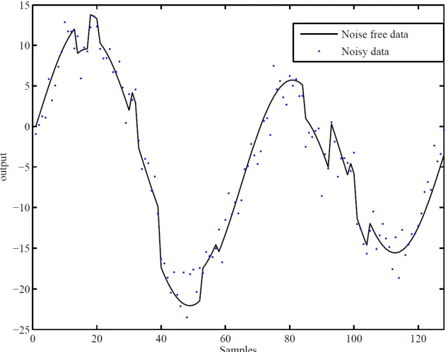
[image:6.595.140.457.457.706.2]

for  . The total number of generated data sam- ples is 128. All variables, inputs and output, are assumed to be noise-free, which are then contaminated with addi- tive zero mean Gaussian noise. Different levels of noise, which correspond to signal-to-noise ratios (SNR) of 10, 20, and 50, are used to illustrate the performances of the various methods at various noise contributions. The SNR is defined as the variance of the noise-free data divided by the variance of the contaminating noise. A sample of the output data, where SNR = 20 is shown in Figure 1.

4.1.2. Simulation Results

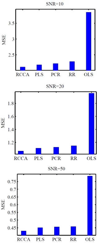
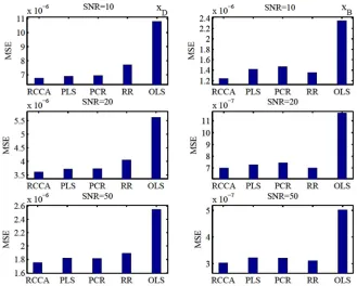
The simulated data are split into two sets: training and testing. The training data are used to estimate inferential models using the various modeling methods, and the testing data are used to compute the model prediction MSE (as shown in Equation (24)) using unseen data. To make statistically valid conclusions about the perform- ances of the various modeling techniques, a Monte Carlo simulation of 1000 realizations is performed and the re- sults are shown in Table 1 and Figure 2. These results show that the performance of RR is better than that of OLS, and that the performances of the LVR modeling techniques (PCR, PLS, and RCCA) clearly outperform the performances of the full rank models (OLS and RR). This is, in part, due to the fact that in LVR modeling, a portion of the noise in the input variables is removed with the neglected principal components, which enhances the model prediction. This is not the case in full rank models (OLS and RR) where all inputs are used to pre- dict the model output. The results also show that the per- formances of PCR and PLS are comparable. These re- sults agree with those reported in the literature [24,25], where the number of principal components is freely op- timized for each model using cross validation and the models predictions are compared using unseen testing data. The optimum numbers of principal components used by the various LVR models for the case where are shown in Figures 3(a), (c) and (e), which show that the optimum number of principal components used in PCR is usually more than what is used in PLS and RCCA to achieve a comparable prediction accuracy. The results in Table 1 and Figure 2 also show that RCCA provides a slight advantage over PCR and PLS when the optimum value of the regularization parameter

a

=20 SNR

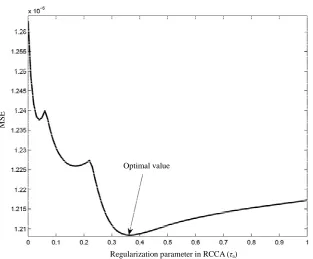
 is used. The value of a is optimized using cross

validation as shown in the RCCA problem formulation given in Equation (22). The optimization of a for one

realization is shown in Figure 4, in which a is opti-

[image:7.595.344.502.84.472.2]

mized by minimizing the cross validation MSE of the estimated RCCA model with respect to the testing data. Note also from Figures3(a), (c) and (e), which compare the number of principal components used by the various

Table 1. Comparison between the prediction MSE’s ob- tained by the various modeling methods with respect to the noise-free testing data.

Model Type SNR = 10 SNR = 20 SNR = 50 RCCA 2.117 1.067 0.4294

PLS 2.183 1.111 0.4510

PCR 2.223 1.127 0.4565

RR 2.288 1.148 0.4584

[image:7.595.55.288.638.735.2]

OLS 3.849 1.955 0.7853

Figure 2. Histograms comparing the prediction MSE’s for the various modeling techniques and at different signal-to- noise ratios.

modeling methods, that RCCA is capable of providing this improvement using a smaller number of principal components than PCR and PLS.

4.1.3. Effect of Scaling the Data on the Predictions and Dimensions of Estimated Models

(a) (b)

(c) (d)

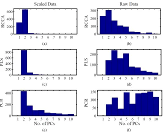
[image:8.595.136.462.82.346.2]

(e) (f)

Figure 3. Histograms comparing the optimum number of principal components used by the various modeling techniques for scaled and raw data for the case where SNR = 20.

Optimal value

Regularization parameter in RCCA (τa)

[image:8.595.147.460.384.630.2]

MSE

Figure 4. Optimization of the RCCA regularization parameter using cross validation with respect to the testing data.

Figure 3, on the other hand, which compares the effect

of scaling on the optimum number of principal compo- nents (for PCR, PLS, and RCCA), shows that when scaled data are used, smaller numbers of PCs are needed for all model estimation techniques, and that RCCA uses the least number of PCs among all techniques.

4.2. Example 2: Inferential Modeling of Distillation Column Compositions

4.2.1. Process Description

The column used in this example, which is simulated using Aspen Plus, consists of 32 theoretical stages (inclu- ding the reboiler and a total condenser). The feed stream, which is a binary mixture of propane and isobutene, en- ters the column at stage 16 as a saturated liquid. The feed stream has a flow rate of 1 kmol/s, a temperature of 322 K, and a propane composition of 0.4. The nominal steady state operating conditions of the column are presented in the Table 2.

4.2.2. Data Generation

The data used in this modeling problem are generated by perturbing the flow rates of the feed and the reflux streams from their nominal operating conditions. First,

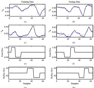
step changes of magnitudes ±2% in the feed flow rate around its nominal condition are introduced, and in each case, the process is allowed to settle to a new steady state. After attaining the nominal conditions again, similar step changes of ±2% in the reflux flow rate around its nomi- nal condition are introduced. These perturbations are used to generate training and testing data (each consist- ing of 64 data points) to be used in developing the vari- ous models. These perturbations (for the training and testing data sets) are shown in Figures6(e)-(h).

[image:9.595.139.460.276.524.2]

In this simulated modeling problem, the input vari- ables consist of ten temperatures at different trays of the column, in addition to the flow rates of the feed and re- flux streams. The output variables, on the other hand, are the compositions of the light component (propane) in the

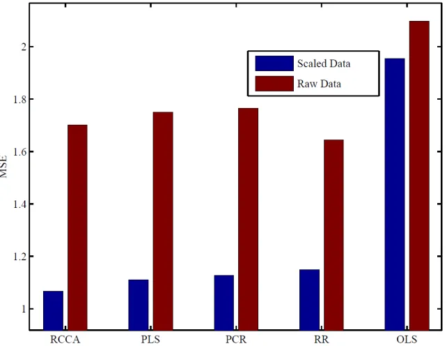
Figure 5. Comparison between the prediction MSE’s of the various modeling techniques using scaled and raw data for the case where SNR = 20.

Table 2. Steady state operating conditions of the distillation column.

Process Variable Value Process Variable Value

Feed

F 1 kg·mole/sec P 1.7022 × 106 _Pa

T 322 K xD 0.979

P 1.7225 × 106 _{Pa Reboiler Drum}

zF 0.4 B 0.5979 kg·mole/sec

Reflux Drum Q 2.7385 × 107 _Watts

D 0.40206 kg·mole/sec T 366 K

T 325 K P 1.72362 × 106 Pa

[image:9.595.56.538.577.736.2]

(a) (b)

(c) (d)

(e) (f)

[image:10.595.133.461.83.388.2]

(g) (h)

Figure 6. Sample data sets showing the changes in the feed and reflux flow rates and the resulting dynamic changes in the distillate and bottom stream compositions; For the composition data—solid line: noise-free data, dots: noisy data, SNR = 20.

distillate and bottom streams (i.e., xD and xB, respec-

tively). The dynamic temperature and composition data generated using the Aspen simulator (due to the pertur- bations in the feed and reflux flow rates) are assumed to be noise-free, which are then contaminated with zeros mean Gaussian noise. To assess the robustness of the various modeling techniques to different noise contribu- tions, different levels of noise (which correspond to sig- nal-to-noise ratios of 10, 20 and 50) are used. Sample training and testing data sets showing the effect of the perturbations on the column compositions are shown in

Figures 6(a)-(d) for the case where the signal-to-noise

ratio is 20.

4.2.3. Simulation Results

The simulated distillation column data (training data and testing) used in this example are scaled as discussed in Example 1. The training data set are used to estimate the model, while the testing data are used to optimize and validate the quality of the estimated models. As per- formed in example 1, the number of principal compo- nents (in the case of LVR techniques, i.e., PCR, PLS, and RCCA) and other parameters (such as the regularization parameters, i.e., λ in RR or a in RCAA) are deter-

mined by minimizing the cross validation MSE for the

To obtain statistic

unseen testing data.

ally valid conclusions about the per- formances of the various modeling techniques, a Monte Carlo simulation of 1000 realizations is performed, and the results are presented in Figure 7 and Table 3. These results show that, in general, the LVR modeling methods (PCR, PLS, and RCCA) outperform the full rank meth- ods (OLS and RR). The results also show that the per- formances of PCR and PLS are comparable, and that by optimizing its regularization parameter a, RCCA can

provide an improvement over these te hniques. The value of a

c

 is optimized using cross validation as shown in th RCCA problem formulation given in Equa- tion (22). The optimization of a

e

 for one realization for the output xD is shown in Figure 8. Finally, the results

show that t prediction abilities of all modeling tech- niques degrade for larger noise contents, i.e., for smaller signal-to-noise ratios. The results obtained in this distil- lation column example agree with the results obtained in Example 1.

he

5. Conclusion

are very commonly used in practice to

theoretical review, an extension to optimize RCCA for Inferential models

[image:11.595.133.462.83.347.2]

Figure 7. Histograms chart comparing the prediction MSE’s of the various modeling techniques using the distillation column data.

3. Comparison between the prediction MSE’s (with respect to the noise-free testing data) of the distillate and bottom ream compositions for the various modeling techniques and at different signal-to-noise ratios.

Table st

output-xD output-xB

Model Type

SNR = 10 (×106_{) SNR = 20 (×10}6_{) SNR = 50 (×10}6_{) SNR = 10 (×10}6_{) SNR= 20 (×10}7_{) SNR = 50 (×10}7₎

RCCA 6.7717 3.6050 1.7532 1.2393 6.9890 3.0253 PLS 6.9062 3.7153 1.8206 1.4192 7.2797 3.2215 PCR 6.9606 3.7237 1.8117 1.4707 7.4419 3.2046 RR 7.706 4.0508 1.8929 1.1979 7.0000 3.1120 OLS 10.787 5.6261 2.549 2.3522 11.670 5.017

enhan diction, l as a com e analysis r various inferential modeling techniques, which in-

gression ( chniques R, PLS, and RCCA) outperform the full rank techniques (i.e., OLS and RR). ced pre as wel parativ

fo

clude ordinary least square (OLS) regression, ridge re- gression (RR), principal component regression (PCR), partial least square (PLS), and regularized canonical cor- relation analysis (RCCA). The theoretical review shows that the loading vectors used in LVR modeling can be computed by solving eigenvalue problems. For RCCA, it is shown that it can be optimized (to provide enhanced prediction ability) by optimizing its regularization pa- rameter, which can be performed by solving a nested optimization problem. The various inferential modeling techniques are compared through two examples, one us- ing synthetic data and the other using simulated distilla- tion column data, where the distillate and bottom stream compositions are estimated using other easily measured variables. Both examples show that the latent variable

This is due to their ability to improve the conditioning of the model by neglecting principal components with small re LVR) te (i.e., PC

eigenvalues, and thus reducing the effect of noise on the model prediction. The obtained results also show that the performances of PCR and PLS are comparable when the number of principal components used are freely opti- mized using cross validation. Finally, it is shown that by optimizing its regularization parameter, RCCA can pro- vide an improvement (in terms of its prediction MSE) over PCR and PLS using a smaller number of principal components.

6. Acknowledgements

[image:11.595.57.539.412.523.2]

Optimal value

Regularization parameter in RCCA (τa)

MS

[image:12.595.143.456.81.340.2]

E

Figure 8. Optimization of the RCCA regularization parameter using cross validation with respect to the testing data.

09-530-2-199 from the Qatar National Research Fund (a mem

ere

“D opment of Inferential Process Models Using PLS,”

puters & Chem 8, No. 7, 1994, pp 597-611. doi:10.1016/0098-1354(93)E0006-U

ber of Qatar Foundation). The statements made in are solely the responsibility of the authors.

h

REFERENCES

[1] J. V. Kresta, T. E. Marlin and J. F. McGregor, evel-

Com-

.

ical Engineering, Vol. 1

[2] R. Weber and C. B. Brosilow, “The Use of Secondary Measurement to Improve Control,” AIChE Journal, Vol. 18, No. 3, 1972, pp. 614-623. doi:10.1002/aic.690180323 [3] B. Joseph and C. B. Brosilow, “Inferential Control Proc-

esses,” AIChE Journal, Vol. 24, No. 3, 1978, pp. 485-509. doi:10.1002/aic.690240313

[4] M. Morari and G. Stephanopoulos, “Optimal Selection of Secondary Measurements within the Framework of State Estimationin the Presence of Persistent Unknown Distur- bances,” AIChE Journal, Vol. 26, No. 2, 1980, pp. 247- 259. doi:10.1002/aic.690260207

[5] I. Frank and J. Friedman, “A Statistical View of Some Chemometric Regression Tools,” Technometrics, Vol. 35, No. 2, 1993, pp. 109-148.

doi:10.1080/00401706.1993.10485033

th Collinearity in Fir Models

Using Bayesian Shrinkage,” Industrial and Engineering

Chemistry Research, Vol. 45, 2006, pp. 292-298.

[6] A. Hoerl and R. Kennard, “Ridge Regression Based Es- timation for Nonorthogonal Problems,” Technometrics, Vol. 8, 1970, pp. 27-52.

[7] J. McGregor, T. Kourti and J. Kresta, “Multivariate Iden- tification: A Study of Several Methods,” IFAC ADCHEM

Proceedings, Toulouse, Vol. 4, 1991, pp. 145-156. [8] M. N. Nounou, “Dealing wi

doi:10.1021/ie048897m

[9] B. R. Kowalski and M. B. Seasholtz, “Recent Develop- ments in Multivariate Calibration,” Journal of Chemom- etrics, Vol. 5, 1991, pp. 129-145.

doi:10.1002/cem.1180050303

[10] M. Stone and R. J. Brooks, “Continuum Regression: Cross-Validated Sequentially Constructed Prediction Em- bracing Ordinaryleast Squares, Partial Least Squar Principal Components Re

es and gression,” Journal of the Royal

ct Observations,”

El-Statistical Society B, Vol. 52, No. 2, 1990, pp. 237-269. [11] S. Wold, “Soft Modeling: The Basic Design and Some

Extensions, Systems under Indire sevier, Amsterdam, 1982.

[12] E. Malthouse, A. Tamhane and R. Mah, “Non-Linear Par- tial Least Squares,” Computers and Chemical Engineer-

ing, Vol. 21, 1997, pp. 875-890. doi:10.1016/S0098-1354(96)00311-0

[13] H. Hotelling, “Relations between Two Sets of Variables,”

Biometrika, Vol. 28, 1936, pp. 321-377.

[14] F. R. Bach and M. I. Jordan, “Kernel Independent Com-

taylor, “Canonical Cor- pplication to Learn- ponent Analysis,” Journal of Machine Learning Research, Vol. 3, No. 1, 2002, pp. 1-48.

[15] S. S. D. R. Hardoon and J. Shawe relation Analysis: An Overview with A

ing Methods,” Neural Computation, Vol. 16, No. 12, 2004, pp. 2639-2664. doi:10.1162/0899766042321814 [16] M. Borga, T. Landelius and H. Knutsson, “A Unified

Compositions from Multiple Temperature Measurements Using Partial Least Squares Regression,” Industrial & Engineering Chemistry Research, Vol. 30, 1991, pp. 2543-2555. doi:10.1021/ie00060a007

[18] M. kano, K. Miyazaki, S. Hasebe and I. Hashimoto, “In- ferential Control System of distillation Compositions Us- ing Dynamicpartial Least Squares Regression,” Journal

of Process Control, Vol. 10, No. 2, 2000, pp. 157-166. doi:10.1016/S0959-1524(99)00027-X

[19] T. Mejdell and S. Skogestad, “Composition Estimator in a Pilot-Plant Distillation Column,” Industrial & Engineer-

ing Chemistry Research, Vol. 30, 1991, pp. 2555-2564. doi:10.1021/ie00060a008

[20] Y. Hiroyuki, Y. B. Hideki, F. C. E. O. Hiromu and F. Hideki, “Canonical Correlation Analysis for Multivariate Regression and Its Application to Metabolic Fingerprint ing,” Biochemical Engineering Journa

- ,

l, Vol. 40, No. 2

echniques,” Lecture Notes in

ol. 3940, 2006, pp. 34-51.

2008, pp. 199-204.

[21] R. Rosipal and N. Kramer, “Overview and Recent Ad-vances in Partial Least Squares. Subspace, Latent Struc-ture and FeaStruc-ture Selection T

Computer Science, V doi:10.1007/11752790_2

[22] P. Geladi and B. R. Kowalski, “Partial Least Square Re- gression: A Tutorial,” Analytica Chimica Acta, Vol. 185, No. 1, 1986, pp. 1-17.

doi:10.1016/0003-2670(86)80028-9

. 20, No. 4, 1978, p. 397. 3

[23] S. Wold, “Cross-Validatory Estimation of the Number of Components in Factor and Principal Components Mod- els,” Technometrics, Vol

doi:10.1080/00401706.1978.1048969

l. 31,

etrics and Intelligent Laboratory Sys-

[24] O. Yeniay and A. Goktas, “A Comparison of Partial Least Squares Regression with Other Prediction Methods,”

Hacettepe Journal of Mathematics and Statistics, Vo 2002, pp. 99-111.

[25] P. D. Wentzell and L. V. Montoto, “Comparison of Prin- cipal Components Regression and Partial Least Square Regression through Generic Simulations of Complex Mixtures,” Chemom

tems, Vol. 65, 2003, pp. 257-279. doi:10.1016/S0169-7439(02)00138-7

ppendix A. Determining the Loading

A

Vectors Using PCR

tarting with the optimization problem shown in Equa-



=1, ,



T

i i

i i

i m

XX

a C a 

the Lagrangian function for this optimization problem can be written as:



_i,



 _iT _{XX i}_i



1 T_{i i}



. S

tion (9), i.e.,

ˆ =argi max

a

. . 1,

i T

s t 

a

a a

(A.1)

L a a C a a a (A.2) Taking the partial derivative of L with respect to ai

and equating it to 0, we get,

2 2  0

L _{  }

C a a (A.3

llo ue problem: ˆ_{i i i}ˆ

i i i

i

 XX

a

which gives the fo wing eigenval





XX

C a a

i.e., the loading vectors used in PCR are the eigenvectors (A.4)

of the covariance matrix CXX.

Appendix B. Determining

oblem shown in Equa-

T i

the Loading

Vectors Using PLS

Starting with the optimization pr

arg max tion (14), i.e.,

ˆ_i

. . 1. i T

s t _{i i}

Xy

a C

the Lagrangian function can be written as follows:







, T 1 T .

i i  i Xyi  i i



L a a C a a (B.2)

of L

a

a a

(B.1)

a

Taking the partial derivative with respect to ai

0 we get, and equating it to

2 _{i i} 0

i



 _{  }

 Xy

L _{C a} a

ˆ

i i

(B.3)

which gives the following eigenvalue problem,

  Xy C a whe (B.4)

re, _i2_i. Multiplying Equation (B.4) by aˆ_i and enforcing the constraint (a aˆ ˆT_{i i}1), we get,

T T

T

ˆ_{i Xy} _{i i}ˆ ˆ_i _i

a C a a (B.5) Taking the transpose of Equation (B.5), we get,

ˆ_i _i.

yX

C a (B.6) Combing Equations (B.4) a

genvalue p

ˆ_i

yXa (B.7)

Appendix C. Determining the

V

Starting with the optimization tio

. . 1

i

T i T

i i

s t 

nd (B.6), we get the fol- lowing ei roblem:

2_{ˆ .}

i i  Xy

C C a

Loading

ectors Using CCA

problem shown in Equa- n (18), i.e.,

ˆ arg maxi  Xy a

XX

a C

a C a a

the Lagrangian function can be written as:



i, i



Ti Xyi



1 Ti XX i



.

L a a C a C a (C.2)

Taking the partial derivative of L with respect to a and equating it to

i

0 we get, 2 _i

i





 

 Xy XX

L

C C

a

1 _ˆ

i i

0,

i 

a (C.3)

which gives the following solution,



 _

XX Xy

C C a (C.4) where _i 2 ._i Multiplying Equation (C.4) by ˆ_iT XX

t,

ˆ_i ˆ_{i i}.

a C

and enforcing the constraint (i.e., a Cˆ_iT _XXaˆ_i1 ), we ge ˆT_i _i TC a_XX  (C.5) Taking the transpose of Equation (C.5), we get,

Xy

a C a

ˆ_i_i.

yX

C a (C.6) Combing Equations (C.4) and (C.

genval

ˆ .

i i  a

Appendix D. Determining the Loading

V

Starting with the optimization p tio

a i

 

 

 I



_i,_i



_iT _i 1 _iT



1 _a



 .

6), we get the fol- lowing ei ue problem:

1 _ˆ 2

i

 _

XX Xy yX

C C C a (C.7)

ectors Using RCCA

roblem shown in Equa- n (20), i.e.,

ˆiargmax iT

a a C





. . 1

i

T

i a

s t 

Xy a

XX

a C  a 1

(D.1)

the Lagrangian multiplier function can be written as follows:

  _a  _i

   _   _

L a a C_{Xy } a C_XX I a_

Taking the partial derivative of

(D.2) with respect to a

L _i

and equating it to 0, we get,





2 1_{i a a i} 0,

i

L _{    }

 _{    }

 

 CXy CXX I a

a (D.3

which gives the following solution:

i i

)





1

ˆ

1 _a _a  

    

 CXX I CXy a (D.4)

where _i2_i. Multiplying Equation (D.4) by





ˆ_iT_1_{a XX} _a _

a C I

(i.e.,

and enforcing the constraint





ˆ_iT_1_{a XX} _a _ˆ_i 1

a C I a ), we ge

i i

t:

ˆT .

a CXy (D.5) Taking the transpose of Equation (D.5 we get,

. ),

ˆ_i _i (D.6)

bining Equations (D.4) and get the fol- lowing eigenvalue problem:

1 

(D.7)

yX C a

Com (D.6), we



₁



_ˆ 2 _ˆ.

a a i i i

  

    