Preprint typeset in JHEP style - HYPER VERSION TCDMATH 10-05 HMI-10-03
Konishi operator at intermediate coupling
Sergey Frolov∗†
Hamilton Mathematics Institute and School of Mathematics, Trinity College, Dublin 2, Ireland
Abstract:TBA equations for two-particle states from the sl(2) sector proposed by Arutyunov, Suzuki and the author are solved numerically for the Konishi operator descendent up to ’t Hooft’s couplingλ≈2046. The data obtained is used to analyze the properties of Y-functions and address the issue of the existence of the critical values of the coupling. In addition we find a new integral representation for the BES dressing phase which substantially reduces the computational time.
∗Email: [email protected]
†Correspondent fellow at Steklov Mathematical Institute, Moscow.
Contents
1. Introduction 1
2. Konishi state energy 4
3. Y-functions 9
4. Large λ expansion from the numerical data 16
5. Conclusion 22
6. Appendix 23
1. Introduction
The Thermodynamic Bethe Ansatz (TBA) is an efficient tool to determine the finite-size spectrum of two-dimensional relativistic integrable models [1]. The relevance of the TBA for the AdS5×S5 spectral problem was advocated in [2] where L¨uscher’s
approach [3] was used to relate exponential corrections to string energy to wrapping effects in dual field theory. Its application to a nonrelativistic model requires under-standing thermodynamic properties of a so-called mirror theory [4] which is obtained from the original model by means of a double-Wick rotation. The mirror model of the light-cone AdS5 ×S5 superstring was studied in detail in [4] where, in
particu-lar, the asymptotic spectrum was identified, and the mirror form of the Bethe-Yang equations of [5] was determined.
The major step towards realizing the TBA approach is to formulate a so-called string hypothesis [6] which classifies the states contributing in the thermodynamic limit. TBA equations and the associated Y-system are then readily derived from it, see e.g. [7]. This step was made last year in [8] where the mirror Bethe-Yang equations [4] were used to formulate a string hypothesis for the AdS5 ×S5 mirror
model. This opened a way to derive the corresponding canonical [9, 10, 11] and simplified TBA equations [12].
The TBA equations combined with a certain analytic continuation procedure proposed for relativistic models in [13, 14] can be also used to find energies of ex-cited states.1 The procedure was called the contour deformation trick in [28] because
it basically reduces to deforming the integration contours in ground-state TBA equa-tions while keeping their form untouched. As a result, excited states TBA equaequa-tions differ only by integration contours. For practical applications however one should take the integration contours back to their ground-state positions, and this results in the appearance of state-dependent driving terms in the TBA equations.
The contour deformation trick was used in [28] to analyze two-particle states from the sl(2) sector. It was shown there that two-particle states are divided into infinitely-many classes, each class having its own set of driving terms in the TBA equations. For the Konishi-like states the TBA equations of [28] are believed to be equivalent to those of [11, 29],2 and our numerics strongly supports this.
The TBA equations obtained in [28] were used to derive the five-loop anomalous dimension of the Konishi operator, and to show numerically [33] that the correspond-ing result perfectly agrees with the one recently obtained via the generalized L¨uscher formulae [34]. The analysis in [28, 33] was then extended to prove the agreement analytically first for the Konishi operator [35], and then for an arbitrary twist-two operator [36] reproducing the results in [37].3 For other applications of the TBA approach to the AdS/CFT spectral problem, see [52]-[57].
In a parallel development the TBA equations proposed in [11] were used in [29] to compute anomalous dimension of the Konishi operator up to a relatively large value of the ’t Hooft coupling constant λ≈664. Analyzing the results obtained, the authors of [29] found the following fitting function for the Konishi state energy or, equivalently, for the conformal dimension of the dual Konishi operator
EGKVK (λ) = √4 λ
2.0004 + 1.988√
λ −
2.60
λ +
6.2 λ3/2
. (1.1)
This formula allows one to make four remarkable predictions. First, it predicts that the coefficient c−1 of the leading term in the large λ expansion is equal to 2 which
agrees with the spectrum of string theory in flat space [58] and asymptotic Bethe ansatz considerations [59]. Second, it shows the vanishing of the constant term c0.
Third, it makes a new prediction which disagrees with the semiclassical consideration in [60] that the first nonvanishing subleading coefficient is also equal to 2. And fourth,
2The set of integral equations proposed in [11,29] was named an integral form of the Y-system.
We find this terminology somewhat misleading because these integral equations were not derived from the Y-system conjectured in [30] but were proposed by following the pure TBA approach, that is by using the canonical TBA equations [9, 10, 11], the contour deformation trick [13], and the largeJ asymptotic solution of the system [30]. A derivation of the TBA equations from the Y-system requires understanding the complicated analytic structure of Y-functions, see [9,31,28,32] for some results in this direction.
3The five-loop computations in [34, 37] were based on [38] where the four-loop anomalous
it predicts that up to an overall factor of √4λ the Konishi state energy is a series in 1/√λ. The last prediction in fact agrees with the argumentation in [60] but it disagrees with the considerations in [61] where the free fermion model describing the
su(1|1) sector in the semi-classical approximation was analyzed, and it was shown that the strong coupling expansion for short states is in powers of 1/√4 λ. It is worth noting that this simple model indeed predicts that the constant term in the strong coupling expansion vanishes. The formulae derived in the framework of the free fermion model would definitely get quantum corrections, and if the prediction of [29] is correct it would imply that these corrections drastically change the structure of the strong coupling expansion.
In this paper we reconsider the computation of the Konishi state energy. We solve numerically the excited states TBA equations [28] for the Konishi operator up to ’t Hooft’s couplingλ≈2046, and use the data obtained to analyze the behavior of Y-functions. We use the analysis to address the issue of the existence of the critical values ofλraised in [28]. The consideration in [28] was based on an assumption that the analytic properties of the exact Y-functions would follow those of the large J asymptotic solution, and if this assumption is not realized then the TBA equations of [29,28] formulated for Konishi-like states at weak coupling may be valid for all values of λ. Extrapolating our results we find that the first critical value for the Konishi operator is most probably greater than 5300,λ(1)cr >5300, which is significantly higher
than the estimate based on the large J asymptotic solution that gives λ(1)cr ≈774.
We also find that the contribution of YQ-functions to the Konishi state energy
grows almost linearly with the string tensiong =√λ/2π. If this behavior continues to hold for all values of λ then this would imply that at large λ the exact Bethe root asymptotes to a constant less than 2. This would be drastically different from the asymptotic behavior of the corresponding solution of the Bethe-Yang equations and would, in particular, imply the absence of the critical values for the Konishi operator. This would be a very puzzling scenario because the full spectrum of string theory in flat space can be reproduced already from the Bethe-Yang equations [59], and ifwdoes not asymptote to 2 it would be necessary to explain how the spectrum follows from the TBA equations. In particular, the spectrum degeneracy would be more difficult to explain because Bethe roots of different states would not behave uniformly at strong coupling.
Examining the data obtained, we found convincing evidence in favor of the pre-diction of [29] that the first nonvanishing subleading coefficient c1 of the 1/
4
√
λ term is equal to 2, and the coefficient c2 of the terms 1/
√
λ vanishes. If one cuts the asymptotic series at order 1/λ5/4 and fits our data then the coefficient c
1 appears
to be 2.02±0.02 depending on the fitting interval used. It is clearly reasonable to assume that c1 is equal to 2. Setting c1 = 0, one then finds that c2 =−0.02±0.01
which is obviously very small.
fitting the data with λ >77, one gets the following fitting function for the Konishi state energy
c−1 =c1 = 2, c2 = 0 =⇒ EK(λ) = 2
4
√
λ+ 2
4
√
λ −
3.26
λ3/4 +
2.53
λ +
4.03
λ5/4 , (1.2)
which differs from (1.1) by the presence of the 1/λ term. Thus, the coefficient c4 of
the term 1/λ does not vanish, and we cannot confirm the prediction of [29] that up to an overall factor of√4λthe largeλexpansion of the Konishi state energy is a series in 1/√λ. The vanishing of c2 could be related to the high degree of supersymmetry
of the model as was pointed out in [60].
If on the other hand one follows [29] and assumes from the very beginning that c2 =c4 = 0 then fitting the data withλ >77, one gets the following fitting function
for the Konishi state energy
c2 =c4 = 0 =⇒ EK(λ) =
4
√ λ
2.00005 + 1.992√
λ −
2.73
λ +
7.45 λ3/2
, (1.3)
which obviously is in a very good agreement with (1.1). The coefficients in (1.3) mildly depend on the fitting interval used and, for example, the last coefficient can take values from 6 to 8.
Let us also mention that our numerical results agree with those of [29] with the 0.0015 precision for most values of λ, and this implies the equivalence of the TBA equations of [11] and [28] for Konishi-like states at weak coupling.4
We used in our computation a new integral representation for the BES dressing phase [62] which significantly reduces the computational time.
The paper is organized as follows. In the next section we present the results of the numerical solution of the TBA equations for the Konishi state energy. In section 3 we discuss the properties of Y-functions and estimate the first critical value ofλ. In section 4 we use our data to find the coefficients of the largeλasymptotic expansion. In the appendix we describe the numerical algorithm used for the computation, and present new formulae for various dressing phases and kernels.
2. Konishi state energy
We solve numerically the following equations from [28]: the simplified TBA equations (4.2-4.5) forYM|w,YM|vw, andY±–functions, and the hybrid equations (4.13) forYQ
-functions, and determine the values of the Bethe rootu2 =−u1 ≡wor, equivalently,
the momentum p=p(w) carried by a string particle from the exact Bethe equation
4Since the considerations in [28] and in v.3 of [11] have the same starting point – the mirror
(8.61). The energy of the Konishi state is then given by the following formula
EK(λ) = 2 + 2
r
1 + 4g2sin2 p
2 −
∞
X
Q=1
Z d e p
2π log(1 +YQ), (2.1)
where peis the momentum of a Q-particle of the mirror theory, and g is the string tension related to ’t Hooft’s coupling λ as λ = 4π2g2. The energy is given by
the difference of the two terms – the first one is the contribution coming from the dispersion relation, and the second one is the Y-functions contribution. We denote the contributions asEdisandEY, respectively, so thatEK =Edis−EY. It is clear that
Edis and −EY play the roles of the kinetic and potential energy of the Konishi state
particles. We will also use the notationEYQ for the contribution of a YQ-function to the energy.
It is known that at large values of ’t Hooft’s coupling the energy of the Konishi state can be expanded in an asymptotic series in powers of 1/√4
λ
EK(λ) = 24 √
λ+c0+
c1 4
√
λ + c2
√
λ + c3
λ3/4 +
c4
λ + c5
λ5/4 +· · · , (2.2)
where the leading 2√4λ behavior follows from the string spectrum in flat space [58], and can be reproduced from the asymptotic Bethe ansatz [59]. The coefficient c0 is
believed to be equal to 0 because that is what one gets from both the free fermion model describing thesu(1|1) sector and the asymptotic Bethe ansatz [61] but to our knowledge an honest string theory derivation ofc0is absent. The largeλperturbative
expansion of the light-cone string sigma model (see [63] for a review) allows one to have any of the coefficients ci nonvanishing. It was however argued in [60] that
the coefficient c2 should vanish due to the high degree of supersymmetry of the
model. Moreover, it follows from the fitting function (1.1) for the Konishi state energy obtained by solving the canonical TBA equations [29] that in fact both the coefficientsc2 and c4 vanish, and then it is tempting to speculate that all coefficients
with even indices vanish: c2k= 0.
One of our aims is to demonstrate that the excited state TBA equations of [28] indeed predict that the leading coefficient is 2, and then to understand if one can fix the coefficients ck, and in particular if the numerical data indeed predicts that
c0 =c2 =c4 = 0.
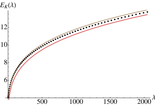
The results of our computation of the Konishi state energy or, equivalently, the conformal dimension of the Konishi operator as a function of g are collected in the table (6.1) from the Appendix. In Figure 1 we plot the data together with the graph of the functionEdis(wasym) wherewasym=wasym(λ) is the corresponding solution of the
Bethe-Yang equation, and the graph of 2√4 λ which is the largeλ asymptote of both the exact and asymptotic energies. One sees that the exact energy graph approaches 2√4
æææ ææ ææ ææ ææ ææ
ææ ææ
ææ ææ
ææ ææ
ææ ææ
ææ ææ
æææ æææ
æææ æ æ ææ æ
æ ææ æ æ ææ æ
æ ææ æ æ ææ æ
æ ææ æ æ æ æ
æ æ
500 1000 1500 2000Λ
6 8 10 12
[image:7.595.169.425.81.260.2]EKHΛL
Figure 1: Black dots represent the numerical solution of the TBA equations for the Konishi state energyEK(λ). The brown (upper) curve represents the solution of the Bethe-Yang equation, and the red (lower) curve is the graph of 2√4
λwhich is the largeλasymptote ofEK(λ). The range of the coupling constant is fromg= 0.1, λ= 0.39 tog= 7.2, λ= 2046.56.
æ ææ ææ
ææ ææ
ææ ææ
ææ ææ
æææ æææ
ææ æ æ ææ æ
æ ææ æ æ ææ æ
æ ææ æ æ ææ æ
æ ææ æ æ ææ æ
æ ææ æ æ ææ æ
æ ææ æ æ ææ æ
æ æ
1 2 3 4 5 6 7 g
6 8 10 12 14 16
EKHgL
Figure 2: Here black dots, the brown and red curves are the same as in Figure 1, and the blue (upper) curve is the graph ofEdis(w) wherew=w(g) is the solution of the exact Bethe equations.
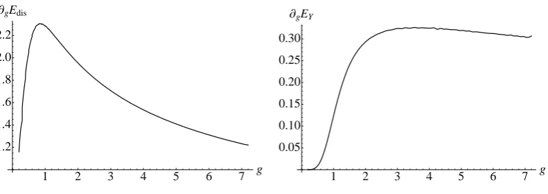
of λ to compare its contribution with the exact energy. The corresponding plots are shown in Figure 2 where we use the string tension g = √λ/2π as an independent variable. We see that Edis(w) grows almost linearly with g for g >4 while the total
energy grows as √g. This implies immediately that the Y-functions contribution also grows linearly, see Figure 3, and, moreover, the linear parts of Edis(w) and EY
cancel each other leading to the √g behavior of EK. On the other hand, Edis(wasym)
grows only as √g for these values of g. It is interesting that the linear dependence of EY becomes clearly visible already at very small values of g. To understand the
reason for such a different behavior of Edis(w) and Edis(wasym) we plot in Figure 4
[image:7.595.169.425.347.511.2]æ æ æ æ æ æ æ æ ææ æ æ ææ æ
ææ ææ
ææ ææ
ææ ææ
ææ ææ
ææ ææ
ææ ææ
ææ ææ
ææ ææ
ææ ææ
ææ ææ
ææ ææ
ææ ææ
ææ ææ
ææ ææ
æ
1 2 3 4 5 6 7 g
0.5 1.0 1.5
[image:8.595.168.425.79.259.2]EYHgL
Figure 3: This is the graph of the contribution ofEY to the energy. It obviously shows a linear
growth starting already withg∼2.
æ
æ
æ æ
æ æææææ
ææ ææ
ææ ææ
ææææ ææææ
ææææ ææææ
æææææææ ææææææ
ææææææææææ ææææææææ
ææææ
1 2 3 4 5 6 7 g 1.5
1.6 1.7 1.8 1.9 2.0 2.1
wHgL
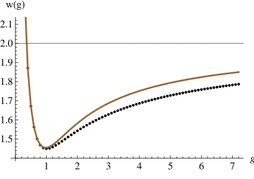
Figure 4: The black dots represent our numerical solution of the exact Bethe equation, and the brown curve is the graph of the corresponding solution of the Bethe-Yang equation. The exact Bethe rootw(g) reaches its minimum atg≈1, andg≈1.6 is the inflection point.
wasym, respectively. The numerical data of the computation of the Bethe root ware
in the table (6.2) in Appendix.
One sees thatwis still pretty far from 2 which is the largegasymptotic value ofwasym,
and that the exact Bethe root is noticably smaller than wasym. The corresponding
exact momentum pis not small at these values of g and decreases much slower than pasym. This explains why the dispersion relation contribution indeed grows as g.
It is tempting to conclude from Figures 2 and 3 thatEdis(w) andEY would grow
[image:8.595.169.425.317.497.2]1 2 3 4 5 6 7 g 1.2
1.4 1.6 1.8 2.0 2.2
¶gEdis
1 2 3 4 5 6 7 g
0.05 0.10 0.15 0.20 0.25 0.30
[image:9.595.102.498.81.221.2]¶gEY
Figure 5: The graphs of the derivative of EdisandEY with respect to g.
equations for Konishi-like states [29, 28] might be valid for any value of g. Also, this would mean that the strong coupling limit of multi-particle states with finite number of particles andJ (short operators in dual field theory) is very different from the near flat space limit discussed in [59, 64] where the rapidities asymptote to 2, and one can study states with J ∼ √g. The puzzle then is that the full spectrum of string theory in flat space can be reproduced already in the near flat space limit [59], and if wdoes not asymptote to 2 it would be necessary to explain how the flat space string spectrum follows from the TBA equations.5
This is an intriguing scenario, and it would be very interesting to understand analytically if it is the one. Our numerics however seems to indicate that the linear growth ofEY might be a feature of the intermediate coupling regime we are studying,
and it will slow down for larger values of g. In Figure 5 we plot the graphs of the derivative of Edis(w) and EY with respect to g (obtained by using the Interpolation
function in Mathematica). We see that the rate of change of EY reaches its
maxi-mum at g ∼3, remains almost constant till g ∼4 and then begins to decrease very slowly. We are not sure if this effect is genuine. The precision of our computation falls down for g > 4, and the decrease in the rate of change of EY may be just a
numerical artifact. Since, as will be discussed in the next section, the contribution of an individual YQ–function to EY slightly decreases at large g it might be also
necessary to include the contribution of more YQ–functions than we did. Then, it is
certainly possible that the rate of change ofEY would stabilize at even larger values
of g, and the scenario discussed above would be realized. The assumption that the Y-functions contribution would be linear in g for very large g has a profound con-sequence on the strong coupling dependence of the Y1–function. Since YQ-functions
are very small for |u|>2 the integration region in (2.1) is effectively of order √g for large g, and, therefore, the Y-functions contribution would grow as g only if logY1
would be of order √g. However, in the next section we will see that it is not the
5Strictly speaking, even ifwasymptotes to 2 but with a rate different from the one of w asym it
0.5 1.0 1.5 2.0 u 5
10 15
Y1Hu,gL; g=1.6, 3.0, 4.4, 5.8, 7.2
1 2 3 4 5 6 7 g 5
10 15
[image:10.595.99.500.81.221.2]Y1H0,gL
Figure 6: On the left figure graphs of fiveY1-functions with different values ofgare shown, and
on the right figure the graph ofY1(0, g) as a function ofg is plotted.
case and for g ∼ 7, Y1 increases only as g3/2. This behavior is different from both
the asymptotic Y1–function g-dependence and the exponential growth required by
the scenario discussed above. This also shows clearly that the values of g we have reached are not large enough, and we are still analyzing the intermediate coupling regime. What happens at larger values of g remains to be understood.
3. Y-functions
In this section we discuss various properties of Y-functions. We begin with YQ -functions because the energy of the Konishi state depends explicitly on them.
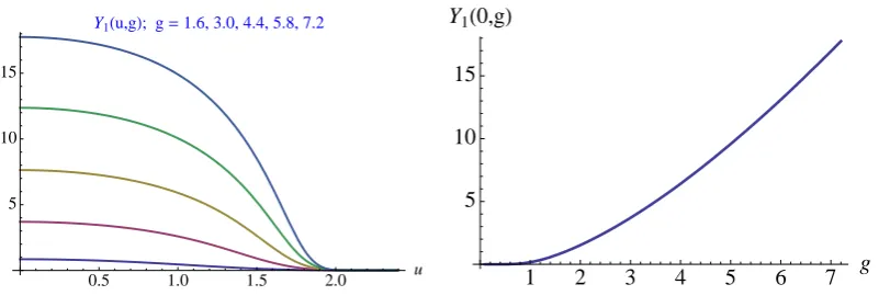
In Figure 6 we show plots6 of several exact Y1-functions computed at various
values of g. One sees that Y1 is getting larger in the interval [−2,2] with g
increas-ing. In fact it increases very fast, and becomes much larger (one order of magnitude) than the asymptotic Yo
1-function computed at the same values of g and w. In
par-ticular, Y1(0, g) keeps increasing while the asymptotic Y1o-function computed with
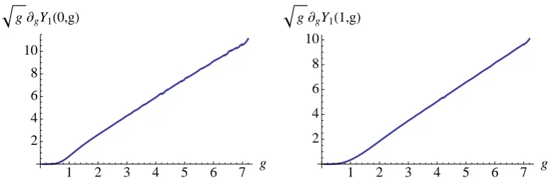
the exact Bethe root w decreases at u = 0 for g > 4. To find the g-dependence we plot √g Y1(0, g) and
√
g Y1(1, g) in Figure 7. We see that they are almost linear
functions, and, therefore, Y1 ∼ g3/2. It is hardly possible that Y1 would show the
g3/2-dependence for large g because this would lead to the contribution of the order
√
glogg to the Konishi state energy which cannot be canceled by any reasonable contribution from Edis. If the exact Bethe root w approaches 2 for large g then
Y1(u, g) should asymptote to a finite function. The existence of the critical values of
g seems to require in addition that Y1(u, g) would go to 0 for anyu <2 (but it could
stay finite for u∼2−ν/g). If w approaches w∞ <2 then, as was mentioned in the previous section, logY1 must grow as
√
g.
In Figure 8 the plot of the contributionEY1 of Y1-function to the Konishi state
energy and the plot of its derivative ∂gEY1 are shown. EY1 decreases too fast to be
1 2 3 4 5 6 7 g 2
4 6 8 10
g¶gY1H0,gL
1 2 3 4 5 6 7 g 2
4 6 8 10
[image:11.595.98.500.82.221.2]g¶gY1H1,gL
Figure 7: The graphs of√g∂gY1(0, g) and
√
g∂gY1(1, g) definitely show that Y1 grows as g3/2.
1 2 3 4 5 6 7 g 0.5
1.0 1.5
EY1
1 2 3 4 5 6 7 g 0.05
0.10 0.15 0.20 0.25
[image:11.595.103.499.270.402.2]¶gEY1
Figure 8: These are the plots ofEY1 and∂gEY1.
[image:11.595.100.499.555.687.2]explained by insufficient numerical precision. The scenario with w∞ < 2 would be realized only if ∂gEY1 asymptotes to a positive constant.
Figure 9 shows plots ofY2-functions. One sees that they exhibit a rather intricate
g dependence. The maximum value of Y2 increases with g and shifts to the right
towardsu= 2.
0.5 1.0 1.5 2.0 u 0.1
0.2 0.3 0.4
Y2Hu,gL; g=1.6, 3.0, 4.4, 5.8, 7.2
1 2 3 4 5 6 7 g 0.01
0.02 0.03
Y2H0,gL
Figure 9: On the left figure graphs of fiveY2-functions with different values ofgare shown, and
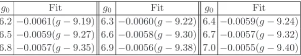
We see from Figure 9 thatY2(0, g) is decreasing forg >3. This behavior agrees
with our expectations based on the analysis of asymptotic Y-functions. Let us recall that Y2-function is one of the Y-functions that can be used to find the first
sub-critical value of g because it vanishes at u = 0 if g = ¯gcr(1) [28]. Let us now assume
that the critical value does exist. Then since Y2 is non-negative for all values ofg it
should have an expansion of the form
Y2(0, g)∼(g−¯gcr(1))
2+· · · .
Since most of our points are far from ¯g(1)cr , to estimate the first sub-critical value we
first however use the linear fit. This would give the lowest estimate7 of the value of ¯
gcr(1) because Y2(0, g) has a double zero at g = ¯g (1)
cr . Fitting our data in the interval
[g0,7.2] to the function c1(g−g¯ (1)
cr ), we get the results shown in (3.1).
g0 Fit g0 Fit g0 Fit
6.2 −0.0061(g−9.19) 6.3 −0.0060(g−9.22) 6.4 −0.0059(g−9.24) 6.5 −0.0059(g−9.27) 6.6 −0.0058(g−9.30) 6.7 −0.0057(g−9.32) 6.8 −0.0057(g−9.35) 6.9 −0.0056(g−9.38) 7.0 −0.0055(g−9.40)
(3.1)
As expected, the estimated value of ¯gcr(1) increases with g0 approaching 7.2, and one
concludes from the table that ¯gcr(1) > 9.4. If on the other hand one fits the data to
c2(g −g¯ (1)
cr )2, one gets
g0 Fit g0 Fit g0 Fit
6.2 0.00061(g−11.66)2 6.3 0.00061(g−11.67)2 6.4 0.00061(g−11.67)2 6.5 0.00061(g−11.68)2 6.6 0.00061(g−11.68)2 6.7 0.00060(g−11.69)2
6.8 0.00060(g−11.70)2 6.9 0.00060(g−11.70)2 7. 0.00060(g−11.71)2
(3.2)
This fitting is much more stable then the linear one, and gives ¯gcr(1) ∼ 11.7. It is
certainly possible that decreasing Y2(0, g) would slow down for larger values of g
resulting in a larger estimate of ¯gcr(1).
The plots of EY2 and ∂gEY2 are shown in Figure 10. The rate of change of
EY2 is still increasing, and one cannot make any reliable prediction about its strong
[image:12.595.138.436.338.394.2]coupling behavior.
Figure 10 shows similar plots ofY3-function. It is still increasing atu= 0 but it
is clear that it will reach its maximum soon.
7We assume there will be no sharp changes in the behavior ofY
1 2 3 4 5 6 7 g 0.05
0.10 0.15 0.20
EY2
1 2 3 4 5 6 7 g 0.01
0.02 0.03 0.04
[image:13.595.97.502.80.219.2]¶gEY2
Figure 10: These are the plots ofEY2 and∂gEY2.
0.5 1.0 1.5 2.0 2.5u 0.01
0.02 0.03 0.04 0.05 0.06
Y3Hu,gL; g=1.6, 3.0, 4.4, 5.8, 7.2
1 2 3 4 5 6 7 g 0.01
0.02 0.03 0.04
[image:13.595.97.504.271.405.2]Y3H0,gL
Figure 11: On the left figure graphs of fiveY3-functions with different values ofgare shown, and
on the right figure the graph ofY3(0, g) as a function ofg is plotted.
Even thoughY3is so small its contribution to the energy is also increasing linearly
withg, see Figure 12, and moreover the rate ofEY3 has already reached its maximum.
1 2 3 4 5 6 7 g 0.01
0.02 0.03 0.04 0.05 0.06 0.07
EY3
1 2 3 4 5 6 7 g 0.005
0.010 0.015
¶gEY3
Figure 12: These are the plots ofEY3 and∂gEY3.
[image:13.595.98.498.518.652.2]0.5 1.0 1.5 2.0u
-0.7
-0.6
-0.5
-0.4
-0.3
-0.2
-0.1
Y-Hu,gL; g=1.6, 3.0, 4.4, 5.8, 7.2
1 2 3 4 5 6 7 g
-0.30
-0.25
-0.20
-0.15
-0.10
-0.05
[image:14.595.98.497.84.205.2]Y-H0,gL
Figure 13: Y−-functions
assumed to have the following expansions8
Y±(0, g)∼g−¯gcr(1)+· · · .
Using again the linear fit, we get the following results forY−(0, g)
g0 Fit g0 Fit g0 Fit
6.2 0.0035(g−8.93) 6.3 0.0034(g−8.98) 6.4 0.0033(g−9.03) 6.5 0.0033(g−9.08) 6.6 0.0032(g−9.13) 6.7 0.0031(g−9.18) 6.8 0.0030(g−9.23) 6.9 0.0030(g−9.28) 7. 0.0029(g−9.33)
(3.3)
The results in the table (3.3) are obviously compatible with those in table (3.1) but the estimated subcritical values ¯gcr(1) in (3.3) appear to be slightly less than
the ones from (3.1). A better estimate of ¯gcr(1) is obtained by fitting the data to
c1(g −g¯ (1)
cr ) +c3(g−g¯ (1) cr )3
g0 Fit g0 Fit
6.2 0.000045(g−11.14)3+ 0.00087(g−11.14) 6.3 0.000043(g−11.19)3+ 0.00085(g−11.19)
6.4 0.000042(g−11.25)3+ 0.00083(g−11.25) 6.5 0.000041(g−11.30)3+ 0.00081(g−11.30) 6.6 0.000040(g−11.36)3+ 0.00079(g−11.36) 6.7 0.000039(g−11.41)3+ 0.00078(g−11.41)
6.8 0.000038(g−11.46)3+ 0.00076(g−11.46) 6.9 0.000037(g−11.51)3+ 0.00074(g−11.51)
(3.4)
with the results similar to those from (3.2).
SinceY+(0, g) is still pretty far from 0 for the values ofg we are dealing with, its
linear extrapolation to larger values ofg would not give very reliable results. Indeed, fitting our data for Y+(0, g) in the interval [g0,7.2] to the linear functionc1(g−g¯
(1) cr ),
we get the results shown in (3.5).
g0 Fit g0 Fit g0 Fit
6.2 0.25(g−9.83) 6.3 0.25(g−9.88) 6.4 0.24(g−9.92) 6.5 0.24(g−9.97) 6.6 0.24(g−10.01) 6.7 0.23(g−10.05) 6.8 0.23(g−10.10) 6.9 0.23(g−10.14) 7. 0.22(g−10.18)
(3.5)
Let us also mention that if one uses c3(g−¯g (1)
cr )3 as a fitting function one gets the
largest of all the estimates: ¯g(1)cr >16.
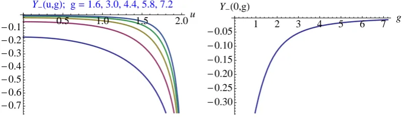
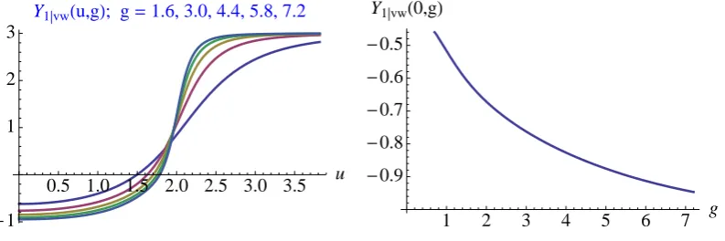
Next we discuss Y1|vw-function, see Figure 15. This is the function that
deter-8It seems possible that the expansion could be of the formY
0.5 1.0 1.5 2.0u
-25
-20
-15
-10
-5
Y+Hu,gL; g=1.6, 3.0, 4.4, 5.8, 7.2
1 2 3 4 5 6 7 g
-8
-6
-4
-2
[image:15.595.98.502.84.209.2]Y+H0,gL
Figure 14: Y+- andY−-functions are approaching 0 atu= 0 withgincreasing. Forg >g¯ (1)
cr they become positive atu= 0, and asymptote to their ground state valueY±gr st= 1 for very largeg.
0.5 1.0 1.5 2.0 2.5 3.0 3.5 u
-1 1 2 3
Y1 vwHu,gL; g=1.6, 3.0, 4.4, 5.8, 7.2
1 2 3 4 5 6 7 g
-0.9
-0.8
-0.7
-0.6
-0.5
Y1 vwH0,gL
Figure 15: Y1|vw-function is approaching−1 at u= 0 withg increasing. It also approaches its ground state value atu=∞faster for largerg.
mines the first critical value ofg because its value atu= 0 has the following behavior in the vicinity of g =g(1)cr
Y1|vw(0, g) + 1∼(g−gcr(1))
2
+· · · .
Using the quadratic fitting functionc2(g−¯g (1)
cr )2, we get the following results
g0 Fit g0 Fit g0 Fit
6.2 0.0028(g−11.52)2 6.3 0.0028(g−11.54)2 6.4 0.0028(g−11.55)2 6.5 0.0028(g−11.57)2 6.6 0.0028(g−11.59)2 6.7 0.0027(g−11.60)2
6.8 0.0027(g−11.62)2 6.9 0.0027(g−11.64)2 7. 0.0027(g−11.65)2
(3.6)
The results in the table (3.6) are compatible with those in table (3.2). For all values of g0 the estimated critical value g
(1)
cr appears to be less than the corresponding
subcritical one from (3.2). They still do not differ much, and it is what one gets from the analysis of asymptotic Y-functions [28].
We conclude from the table (3.6) that gcr(1) > 11.6, and it seems reasonable
to expect that g(1)cr would not exceed 12.0 (it might appear to be a too optimistic
expectation), so the first critical value of λ would be in the interval 5300 < λ(1)cr <
[image:15.595.103.500.264.396.2]0.5 1.0 1.5 2.0 2.5 3.0 3.5 u 2
4 6 8
Y2 vwHu,gL; g=1.6, 3.0, 4.4, 5.8, 7.2
1 2 3 4 5 6 7 g 0.5
1.0 1.5 2.0 2.5
[image:16.595.98.498.84.223.2]Y2 vwH0,gL
Figure 16: Y2|vw-function is approaching 0 at u= 0 with g increasing. It also approaches its ground state value atu=∞faster for largerg.
1 2 3 4 u
10 20 30 40 50 60 70
Y1 wHu,gL; g=1.6, 3.0, 4.4, 5.8, 7.2
1 2 3 4 5 6 7 g 10
20 30 40 50 60 70
Y1 wH0,gL
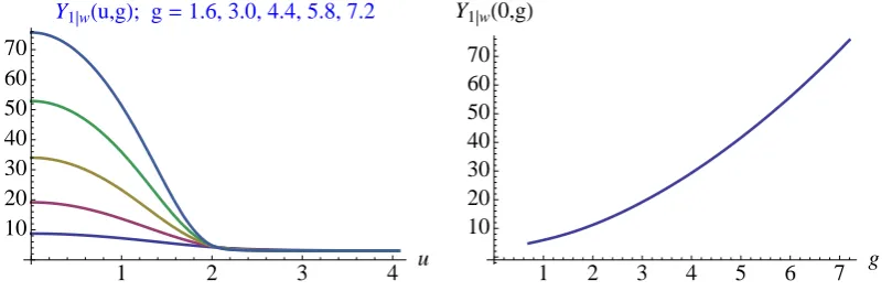
Figure 17: On the left figure graphs of five Y1|w-functions with different values ofg are shown, and on the right figure the graph ofY1|w(0, g) as a function ofg is plotted.
The first subcritical value can be also determined from Y2|vw, see Figure 16, because its value at u= 0 vanishes, and it has the following expansion
Y2|vw(0, g)∼g−¯gcr(1)+· · · .
Y2|vw(0, g) is also pretty far from 0 and its linear extrapolation to larger values of g gives results slightly lower than those from table (3.2)
g0 Fit g0 Fit g0 Fit
6.2 −0.137(g−10.91) 6.3 −0.136(g−10.94) 6.4 −0.135(g−10.97) 6.5 −0.134(g−11.00) 6.6 −0.133(g−11.02) 6.7 −0.132(g−11.05) 6.8 −0.131(g−11.08) 6.9 −0.130(g−11.10) 7. −0.130(g−11.13)
(3.7)
The estimates can be made closer to the previous ones if one fits the data to higher order polynomials.
Let us finally mention thatYw-functions do not show any particularg-dependence.
They just are increasing very fast, see Figure 17.
It is worth stressing that the estimate ofgcr(1)was made under an assumption that
the first critical value exists. If it does not then Y1|vw(0, g) would (or not) approach
[image:16.595.97.502.276.413.2]4. Large
λ
expansion from the numerical data
As was discussed in section 2 at large values of ’t Hooft’s coupling the Konishi state energy admits an asymptotic expansion in powers of 1/√4 λ
EK(λ) =c−1 4
√
λ+c0 +
c1 4 √ λ + c2 √ λ + c3
λ3/4 +
c4
λ + c5
λ5/4 +· · · . (4.1)
In this section we try to understand to what extent our numerical data can be used to fix the coefficients ci. We should point out however that in general an asymptotic series cannot be found reliably from numerical data. For example, the function 21−e1000000−
√
λ
1+e1000000−√λ
4
√
1 +λ obviously asymptotes to 2√4 λ but any numerical computation
performed forλ <1000000 would predict that it asymptotes to−2√4λ. Thus, we have to assume first of all that exponentially suppressed terms become very small already at the values ofλwe are dealing with. Then, a function can approach its asymptotic series monotonically or in oscillations, and it does not seems possible to single out one from numerics. In fact, using the standard least-square fitting procedure would always lead to an oscillating behavior of numerical data about a fitting function. Next, if λ is not large enough then one may need to make an assumption about the structure of the large λ expansion, for example to decide if the series contains all possible terms or some of them vanish. Finally, fitting numerical data one should decide how many terms one should keep in an asymptotic series, and what fitting interval one should use.
Since the precision of our computation is about 10−4 forg ∼7 it seems reasonable
to keep only the terms up to the 1/λ5/4 order in the asymptotic expansion (4.1) . The
fitting is done by using the data with the string tension taking values in the interval [g0, g1] whereg1 changes from 4.0 to 7.2 (with the step 0.1), and Mathematica’s Fit
(or FindFit) functions. The first point of the fitting interval is chosen to beg0 = 1.4,
λ≈77 because it is larger than the inflection point of the Konishi state energy which is ginfl≈0.8, λ≈25.
We begin the fitting by making no assumption about the structure of the large λ expansion. Below we present the table (4.2) where we use the function in (4.1) to fit our numerical results in (6.1).
g1 λ1 Fit
4. 632. 0.0748723−19.5546
λ5/4 − 26.8658
λ3/4 + 1.99888 4
√
λ+0.886704√4λ + 7.23013√
λ +
40.4154
λ
4.4 764. 1.3609−176.565
λ5/4 − 198.245
λ3/4 + 1.94263 4
√
λ−11.2876 4
√
λ +
68√.3193
λ +
295.295
λ
4.8 910. 0.94197−117.655
λ5/4 − 137.196
λ3/4 + 1.96036 4
√
λ−7.19535 4
√
λ +
47√.1638
λ +
202.045
λ
5.2 1070. 0.443739−41.3538
λ5/4 − 60.5348
λ3/4 + 1.98102 4
√
λ−2.23404 4
√
λ +
21√.0468
λ +
83.0606
λ
5.6 1240. −0.0777338 +45λ.56551/4 + 24.2251
λ3/4 + 2.0022 4
√
λ+3.06072√4
λ −
7.33942√
λ −
50.6135
λ
6. 1420. −0.439602 +110.23
λ5/4 + 85.6348
λ3/4 + 2.01667 4
√
λ+6.79178 4
√
λ −
27.√6317
λ −
148.678
λ
6.4 1620. −0.131008 +51λ.5482/4 + 31.0414
λ3/4 + 2.00453 4
√
λ+3.56246√4λ − 9.√8231
λ −
60.4474
λ
6.8 1830. 0.201473−15.5603
λ5/4 − 30.0019
λ3/4 + 1.99163 4
√
λ+0.0366606√4λ + 9.86239√
λ +
39.2596
λ
7.2 2050. 0.210769−17.5595
λ5/4 − 31.7814
λ3/4 + 1.99128 4
√
λ−0.0634158 4
√
λ +
10√.429
λ +
42.2007
λ
æ æ æ æ æ ææ æ ææ æ æ æ æ æ æ æ æ æ
æ æ æ æ
ææ æ
æ ææ æ æ æ æ
4.5 5.0 5.5 6.0 6.5 7.0
g
11.92
1.94
1.96
1.98
c
-1H
g
1L
æ æ æ æ æ æ æ æ æ æ æ æ æ æ æ æ æ æ æ æ ææ
ææ æ
æ æ ææ ææ æ æ
4.5 5.0 5.5 6.0 6.5 7.0
g
10.5
1.0
1.5
2.0
[image:18.595.104.500.84.206.2]c
0H
g
1L
Figure 18: On the left and right figures the graphs ofc−1 andc0 as functions ofg1 are plotted.
The fitting is done without any constraint imposed onci.
To better visualize the results in Figure 18 we also plot the coefficients c−1 and c0.
As one can see, the coefficient c−1 of the leading term is oscillating about 2, and for
g1 >6.2 it is getting quite close to 2. Its average value is 1.983. The coefficient c0 is
oscillating about 0 but it is not really small with the average equal to 0.385. There is however an obvious correlation between the values of c−1 and c0 – the closer c−1
is to 2 the closer c0 is to 0.
The subleading coefficients are however not fixed at all and take very different values depending on the fitting interval used. The fitting therefore is not stable, and the fitting function strongly depends on the fitting interval. One may conclude that the numerical data allows one to fix only the leading coefficient in the strong coupling expansion. One should remember however that the series (4.1) is only asymptotic, and fixing its coefficients by using the data for these not very large values ofλis not that straightforward as it is for a convergent series.
To proceed let us fix the leading coefficient to be 2. Then, fitting the numerical data, one finds the results in table (4.3) and Figure 19.
g1 λ1 Fit
4. 632. 0.0487754−16.0827
λ5/4 − 23.1977
λ3/4 + 2 4
√
λ+1.13832√4
λ +
5.94492√
λ +
34.8688
λ
4.4 764. −0.00945538 +26.2666
λ5/4 + 7.84673
λ3/4 + 2 4
√
λ+2.2426 4
√
λ −
2.36707√
λ −
22.6721
λ
4.8 910. −0.0269174 +40λ.53386/4 + 17.7895
λ3/4 + 2 4
√
λ+2.58159√4λ − 4.97525√
λ −
41.4559
λ
5.2 1070. −0.030125 +43λ.50799/4 + 19.6865
λ3/4 + 2 4
√
λ+2.64471√4λ − 5.46707√
λ −
45.0787
λ
5.6 1240. −0.0216031 +34.8027
λ5/4 + 14.2113
λ3/4 + 2 4
√
λ+2.47195 4
√
λ −
4.08328√
λ −
34.3737
λ
6. 1420. −0.00723624 +20λ.06485/4 + 4.64678
λ3/4 + 2 4
√
λ+2.17693√4λ − 1.69214√
λ −
15.4861
λ
6.4 1620. −0.0115075 +24λ.57422/4 + 7.61427
λ3/4 + 2 4
√
λ+2.√4266λ − 2.42443√
λ −
21.4161
λ
6.8 1830. −0.0230903 +38λ.51119/4 + 15.9437
λ3/4 + 2 4
√
λ+2.√51064
λ −
4.45848√
λ −
38.2204
λ
7.2 2050. −0.0269859 +42.8933
λ5/4 + 18.8607
λ3/4 + 2 4
√
λ+2.59408 4
√
λ −
5.16215√
λ −
44.1706
λ
(4.3)
The coefficient c0 is now much smaller but it stops oscillating about 0. The average
value of c0 is−0.016, and c0 is decreasing with g1 increasing. The subleading
coeffi-cientc1 is not close to 2, it has an average 2.37, and is greater than 2 for almost all
æ æ æ æ æ æ æ æææææ
æ æ æ æ æ æ æ æ ææ æ æ æ æ æ æ
æ æ æ æ
4.5 5.0 5.5 6.0 6.5 7.0
g
1-
0.03
-
0.02
-
0.01
0.01
0.02
c
0Hg
1L
æ æ æ æ æ æ æ æ æ
æææ æ æ æ æ æ æ æ æ ææ æ æ æ æ æ æ æ ææ
æ
4.5 5.0 5.5 6.0 6.5 7.0
g
11.6
1.8
2.2
2.4
2.6
[image:19.595.104.499.84.213.2]c
1H
g
1L
Figure 19: On the left and right figures the graphs of c0 and c1 as functions ofg1 are plotted.
The fitting is done withc−1= 2.
æ æ æ æ æ æ æ æ æ æ æ æ æ æ æ æ æ
ææ æ æ ææ
ææ æ æ æ ææ ææ æ
4.5 5.0 5.5 6.0 6.5 7.0
g
12.02
2.04
2.06
2.08
c
1H
g
1L
æ æ æ æ æ æ æ æ æ ææ ææ æ ææ æææ
æ æ ææ ææ æ ææ ææ ææ æ
4.5 5.0 5.5 6.0 6.5 7.0
g
1-
1.2
-
1.0
-
0.8
-
0.6
-
0.4
-
0.2
[image:19.595.108.498.270.388.2]c
2H
g
1L
Figure 20: On the left and right figures the graphs of c1 and c2 as functions ofg1 are plotted.
The fitting is done withc−1= 2 andc0= 0.
c0 is to 0 the closer c1 is to 2. One sees that for the range of λ we are analyzing
the contribution of the constant term is much smaller than the one of the subleading term c1/
4
√
λ and, therefore, it is reasonable to assume that c0 = 0.
Fixing now the leading and constant coefficients to be 2 and 0, respectively, one finds the results in table (4.4) and Figure 20.
g1 λ1 Fit
4. 632. 22λ.52908/4 + 4.1118
λ3/4 + 2 4
√
λ+2.07902√4
λ −
1.25263√
λ −
16.5214
λ
4.4 764. 18.0024
λ5/4 + 2.18271
λ3/4 + 2 4
√
λ+2.0558 4
√
λ −
0.905321√
λ −
11.8034
λ
4.8 910. 14λ.5458/4 + 0.641502
λ3/4 + 2 4
√
λ+2.03799√4λ − 0.633195√
λ −
7.96653
λ
5.2 1070. 11λ.54777/4 − 0.621309
λ3/4 + 2 4
√
λ+2.02384√4λ − 0.413548√
λ −
4.77967
λ
5.6 1240. 10.2483
λ5/4 − 1.13316
λ3/4 + 2 4
√
λ+2.01824 4
√
λ −
0.325432√
λ −
3.47594
λ
6. 1420. 11λ.52064/4 − 0.748872
λ3/4 + 2 4
√
λ+2.02225√4λ − 0.390144√
λ −
4.47424
λ
6.4 1620. 9.λ648515/4 − 1.36445
λ3/4 + 2 4
√
λ+2.01594√4λ − 0.287401√
λ −
2.86239
λ
6.8 1830. 5.λ808015/4 − 2.85568
λ3/4 + 2 4
√
λ+2.00097√4
λ −
0.041104√
λ +
1.07875
λ
7.2 2050. 2.78511
λ5/4 − 4.00844
λ3/4 + 2 4
√
λ+1.98967 4
√
λ +
0.147219√
λ +
4.15477
λ
(4.4)
It is clear from the table and Figure 20 that fixing c−1 = 2 and c0 = 0 makes the
first nontrivial subleading coefficient c1 to be very close to 2. Its average value is
æ æ
æ ææ
ææ æ æææ æ æ æ æ
ææ æ æ
æ ææ æ æ æ
æ æ æ æ æ æ æ æ
4.5 5.0 5.5 6.0 6.5 7.0
g
1-
0.04
-
0.03
-
0.02
-
0.01
c
2H
g
1L
æ æ æ æ æ æ æ
ææ æ æ æ ææ ææ
æ æ æ
æ æ
æ æ æ æ æ æ æ æ æ æ æ æ
4.5 5.0 5.5 6.0 6.5 7.0
g
1-
3.05
-
3.00
-
2.90
-
2.85
-
2.80
-
2.75
[image:20.595.100.498.84.198.2]c
3H
g
1L
Figure 21: On the left and right figures the graphs of c2 and c3 as functions ofg1 are plotted.
The fitting is done withc−1= 2,c0= 0 andc1= 2.
However c2 is increasing and becomes very close to 0 for g1 = 6.9.
Since the coefficient c1 is so close to 2, let us proceed by fixing c−1 = 2, c0 = 0,
and c1 = 2. Then, one obtains the following table and Figure 21
g1 λ1 Fit
4. 632. 6.la481395/4 −
2.7364 la3/4 + 2
4
√
la + √42la−
0.044888√ la +
0.556775 la
4.4 764. 5.la927115/4 −
2.86533 la3/4 + 2
4
√
la + √42la−
0.0331335√ la +
1.02244 la
4.8 910. 5.63528
la5/4 −
2.93171 la3/4 + 2
4
√
la + √42
la−
0.0271635√ la +
1.26505 la
5.2 1070. 5.57229 la5/4 −
2.94569 la3/4 + 2
4
√
la + 2
4
√ la−
0.0259249√ la +
1.31682 la
5.6 1240. 5.la458785/4 −
2.97011 la3/4 + 2
4
√
la + √42la−
0.0238023√ la +
1.40878 la
6. 1420. 5.la036615/4 −
3.0599 la3/4 + 2
4
√
la + √42la−
0.0160542√ la +
1.749 la
6.4 1620. 5.00365
la5/4 −
3.06689 la3/4 + 2
4
√
la + √42
la−
0.0154523√ la +
1.77553 la
6.8 1830. 5.la512035/4 −
2.96201 la3/4 + 2
4
√
la + √42la−
0.0243275√ la +
1.37154 la
7.2 2050. 6.la080445/4 −
2.84643 la3/4 + 2
4
√
la + √42la−
0.0340167√ la +
0.922834 la
(4.5)
The fitting with the subleading coefficient equal to 2 makes the coefficient c2 to be
very small with the average −0.026. Its contribution to the energy is much smaller than the contribution of the next term c3/λ3/4, and it is reasonable to assume that
c2 is equal to 0. So, let us proceed by fixing c−1 = 2, c0 = 0, c1 = 2, and c2 = 0.
Then, one obtains the following table and Figure 22
g1 λ1 Fit
4. 632. 4.19637 la5/4 −
3.24272 la3/4 + 2
4
√
la + 2
4
√ la +
2.43269 la
4.4 764. 4.la151385/4 −
3.24647 la3/4 + 2
4
√
la + √42la +
2.45884 la
4.8 910. 4.la111455/4 −
3.24973 la3/4 + 2
4
√
la + √42la +
2.48182 la
5.2 1070. 4.05719 la5/4 −
3.25408 la3/4 + 2
4
√
la + 2
4
√ la +
2.51283 la
5.6 1240. 4la.01545/4 −
3.2574 la3/4 + 2
4
√
la + √42la +
2.5366 la
6. 1420. 4.la029855/4 −
3.25628 la3/4 + 2
4
√
la + √42la +
2.52846 la
6.4 1620. 4.00445
la5/4 −
3.25825 la3/4 + 2
4
√
la + √42
la + 2.54273
la
6.8 1830. 3.89399 la5/4 −
3.26672 la3/4 + 2
4
√
la + 2
4
√ la +
2.60457 la
7.2 2050. 3.la758395/4 −
3.27702 la3/4 + 2
4
√
la + √42la +
2.68017 la
(4.6)
We see an interesting effect of this fitting. It appears to be rather stable. As one can see from the table (4.5), the remaining three coefficients c3,c4 and c5 are not in
ææ æææ ææ
æ æ æ æ æ æ æ
æ æ æ æ æ
æ æ æ ææ æ æ æ æ æ æ æ æ æ
4.5 5.0 5.5 6.0 6.5 7.0
g
1-
3.275
-
3.270
-
3.265
-
3.260
-
3.250
-
3.245
c
3Hg
1L
ææ æ
ææ æ ææ
ææ æ
ææ ææ æ
ææ æ æ æ æ ææ
æ æ æ æ æ æ æ æ æ
4.5 5.0 5.5 6.0 6.5 7.0
g
12.45
2.50
2.55
2.60
2.65
[image:21.595.106.497.84.203.2]c
4H
g
1L
Figure 22: On the left and right figures the graphs of c2 and c3 as functions ofg1 are plotted.
The fitting is done withc−1= 2,c0= 0 andc1= 2.
To continue we use the average value of c3, and fit the coefficients c4 and c5.
Then, we use the average value of c4, and fit the coefficient c5. Finally, taking the
average value of c5, we find the following fitting function
g0 = 1.4 : EK(λ) = 2
4
√
λ+ √42
λ −
3.26
λ3/4 +
2.53
λ +
4.03
λ5/4 . (4.7)
Obviously, the fitting function is different from (1.1), in particular the coefficient c4
is not small and gives a significant contribution to the energy. The coefficients ci in
(4.7) depend on the choice of g0. In the table below we present fitting functions for
1.2≤g0 ≤1.6
g0 EK
1.2 2√4λ+ √42
λ − 3.18 λ3/4 +
1.89
λ +
5.27 λ5/4
1.3 2√4λ+ √42λ −
3.22 λ3/4 +
2.25
λ +
4.57 λ5/4
1.4 2√4
λ+ √42
λ − 3.26 λ3/4 +
2.53
λ +
4.03 λ5/4
1.5 2√4λ+ √42
λ − 3.27 λ3/4 +
2.63
λ +
3.83 λ5/4
1.6 2√4λ+ √42
λ − 3.28 λ3/4 +
2.70
λ +
3.69 λ5/4
(4.8)
One can see that onlyc3is relatively stablec3 =−3.23±0.05 but the other coefficients
change more substantially.
Does our fitting rule out the strong coupling expansion in powers of 1/√λ ad-vocated in [29]? In Figure 23 we compare the fitting functionEK(λ) (4.7) with two
fitting functions obtained by setting c2k = 0 from the very beginning. Both EK(λ)
and the function (1.3) fit the data equally well. This is not surprising because both functions have the same number of free fitting parameters. On the other hand, the function EGKVK (λ) = 2√4 λ+ √42
λ − 2.94 λ3/4 +
8.83
λ5/4 obtained by setting c−1 = c1 = 2 and
c2k = 0 significantly deviates from the data, up to 0.0002, which is at least twice
more than the precision of our computation for g < 5. Thus, we are to conclude that the coefficient c4 does not vanish and the strong coupling expansion is in
pow-ers of 1/√4
æ
æ
ææææææææææææææææææææ
ææææææææææææææææææææææææææææææ æææææ
æææ
à à à à à à àààààààà
à àà à àà ààà à ààààà ààààà
àààààà àààààààààààà
ààààà
ààà
0 2 3 4 5 6 7 g
-0.0004
-0.0002 0.0002
DEKHgL
æ æ ææ æ æææ æ ææææ æææ æ æ æ æ æ æ æ æ æ ææ æ æ æ
æææææ æ æ ææ æ æ ææ æ æ æ æ æ æææ æ ææ æ æ æ æ æ àà à àà àà à à à à àà ààà à à à à à à à à à àà à à à àààààà à à à à à àà à à à à à ààà à àà à à à à à
0 2 3 4 5 6 7 g
-0.00005 0.00005
[image:22.595.105.499.79.216.2]DEKHgL
Figure 23: Black dots represent the difference between the computed values of the Konishi energy and its fitting function (4.7): ∆EK =EK −EK. Green squares on the left picture represent a similar difference with EGKVK where the fitting function E
GKV
K (λ) = 2
4
√
λ+ √42λ −
2.94
λ3/4 +
8.83
λ5/4 is obtained by using our data and setting c−1 =c1 = 2 andc0 =c2 =c4 = 0. On the right picture
green squares represent the difference ofEK and the fitting function in (1.2).
æ
æ æ
æ æ
æ æ æ
æ æ æ æ æ æ
0.2 0.4 0.6 0.8 1.0 1.2 1.4
g
1
2
3
4
E
K-
2
Λ
14æ
æ æ
æ
æ æ
æ æ æ æ æ æ æ æ
0.2 0.4 0.6 0.8 1.0 1.2 1.4
g
1
2
3
4
E
K-
2
Λ
14Figure 24: Black dots represent the difference between the energy and its leading largeλ asymp-totic, EK−2
4
√
λ. Red (upper) curve is the graph of EK−2
4
√
λ. Green curve on the left picture is the graph of EGKVK (λ)−2
4
√
λ, and on the right picture it is the difference between the fitting function (1.3) and 2√4
λ. The red curve works very well starting already withg= 0.3, λ= 3.55.
computation for g ∼ 7.0 is not 0.0001 but about 0.0002, and if the contribution of exponentially suppressed terms is of order 0.0002 for g ∼2, then this could explain the left plot on Figure 23 and make possible the vanishing of c4.
Let us finally mention that the functionEK works unexpectedly well (and better than EGKVK or (1.3)) starting already with such a small value of the coupling con-stant as g = 0.3, λ = 3.55, see Figure 24, that is less than the expected radius of convergency of the weak-coupling expansion, even though the fitting was done for the data with g ≥1.4. This implicitly confirms that c1 = 2. Since
4
√
3.55 = 1.37 is close to 1, changingc1just by 0.1 would require an essential change of the coefficients
c3, c4 and c5 to fit the energy data at large λ but then the fitting at small λ would
be destroyed.
[image:22.595.91.508.312.451.2]æ ææ æ æ æ
æ ææ
æ æ
æ æ
æ æ
æ æ æ æ
æ æ
æ æ
æ æ
æ æ
æ æ
æ æ
æ æ æ
æ æ
æ æ
æ æ
æ
1 2 3 4 g
-0.0015
-0.0010
-0.0005 0.0005 0.0010 0.0015
[image:23.595.170.425.84.239.2]EKHgL-EKGKVHgL
Figure 25: The black dots represent the difference between the values of the Konishi energy we obtained and those from [29]. One sees that our results agree with those of [29] with 0.0015 precision for almost all values ofg.
5. Conclusion
In this paper we solved the TBA equations for the Konishi operator descendent from the sl(2) sector proposed by Arutyunov, Suzuki and the author [28] up to ’t Hooft’s coupling λ ≈ 2046. At this value the iterations converge very slowly. It would be important to improve the numerical algorithm and approach closer to the first critical value of λ, and go beyond it. One possible improvement would be to use Newton’s method for solving the TBA equations as it was done for the Hubbard model in [65]. Solving the TBA equations numerically for large values ofλis a challenging problem also because at large λ the Konishi state energy is very close to the energy of the other two Konishi-like states with n = 1, see [28] for detail. It would be interesting to repeat the computation for these states, and for other Konishi-like states with larger string levels.
Fitting the data for the Konishi state energy9 we found convincingly that the
first nontrivial subleading coefficient c1 is equal to 2 and the coefficient c2 vanishes
in agreement with the previous prediction [29]. The coefficient c4 however does not
vanish and therefore the strong coupling expansion seems to be not in powers of 1/√λ (up to an overall √4
λ) but in powers of 1/√4
λ.
In principle increasing the values of λ may change the fitting coefficients and invalidate the predictions for the coefficients. It is necessary to derive them by analytic means.
Extrapolating the results obtained shows that the first critical value for the Konishi operator is λ(1)cr >5300 and it is probably in the range 5300 < λ(1)cr < 5700
which is significantly higher than the estimate based on the large J asymptotic
9We assumed the absence of logλ-dependent terms in the asymptotic largeλexpansion. These
solution that gives λ(1)cr ≈ 774. This means that even at such a large value of λ we are still far from the strong coupling regime. This is an intermediate coupling regime and in fact it is the one where YQ-functions play the most important role. Moreover, if the contribution of YQ-functions to the Konishi state energy will continue growing as √λ then this would imply that at large λ the exact Bethe root asymptotes to a constant less than 2, and the critical values for the Konishi operator are absent.
It is clear that the numerical computation we performed raised more questions than gave answers. Some of the questions can be answered only analytically, and we hope to address them in future.
Acknowledgements
The author thanks Gleb Arutyunov, Zoltan Bajnok, Niklas Beisert, Davide Fiora-vanti, Tristan McLoughlin, Jan Plefka, Radu Roiban, Matthias Staudacher, Ryo Suzuki, Roberto Tateo, Arkady Tseytlin and Kostya Zarembo for interesting discus-sions and comments on the manuscript, and Dmitri Grigoriev for computer help. This work was supported in part by the Science Foundation Ireland under Grants No. 07/RFP/PHYF104 and 09/RFP/PHY2142, and by a one-month Max-Planck-Institut f¨ur Gravitationsphysik Albert-Einstein-Institut grant.
6. Appendix
Numerical data
Here we collect our numerical data.
In the table (6.1) we present the results of the computation of the energy of the Konishi state or, equivalently, the conformal dimension of the Konishi operator as a function of g
g EK g EK g EK g EK g EK g EK
0.1 4.02971 0.2 4.11551 0.3 4.24885 0.4 4.41886 0.5 4.61469 0.6 4.82682 0.7 5.04775 0.8 5.27151 0.9 5.49399 1. 5.71265 1.1 5.92614 1.2 6.13385 1.3 6.33561 1.4 6.53156 1.5 6.72212 1.6 6.90752 1.7 7.0881 1.8 7.2642 1.9 7.43612 2. 7.60411 2.1 7.76844 2.2 7.92935 2.3 8.08702 2.4 8.24163 2.5 8.39336 2.6 8.54238 2.7 8.68879 2.8 8.83276 2.9 8.97441 3. 9.11381 3.1 9.2511 3.2 9.38638 3.3 9.51969 3.4 9.65117 3.5 9.78087 3.6 9.90884 3.7 10.0352 3.8 10.1599 3.9 10.2831 4. 10.4049 4.1 10.5252 4.2 10.6442 4.3 10.7618 4.4 10.8782 4.5 10.9933 4.6 11.1072 4.7 11.22 4.8 11.3316 4.9 11.4421 5. 11.5516 5.1 11.66 5.2 11.7675 5.3 11.8739 5.4 11.9794 5.5 12.084 5.6 12.1877 5.7 12.2905 5.8 12.3924 5.9 12.4936 6. 12.5938 6.1 12.6933 6.2 12.792 6.3 12.89 6.4 12.9872 6.5 13.0837 6.6 13.1795 6.7 13.2746 6.8 13.369 6.9 13.4627 7. 13.5558 7.1 13.6483 7.2 13.7401
In the table (6.2) we present the results of the computation of the Bethe root w
g wK g wK g wK g wK g wK g wK
0.1 5.88827 0.2 3.11236 0.3 2.25445 0.4 1.87021 0.5 1.67116 0.6 1.56174 0.7 1.50066 0.8 1.46819 0.9 1.45317 1. 1.4489 1.1 1.45121 1.2 1.45758 1.3 1.46638 1.4 1.47661 1.5 1.48748 1.6 1.49866 1.7 1.50987 1.8 1.52093 1.9 1.53174 2. 1.54224 2.1 1.55239 2.2 1.56217 2.3 1.57159 2.4 1.58064 2.5 1.58934 2.6 1.59769 2.7 1.60569 2.8 1.61339 2.9 1.62078 3. 1.62787 3.1 1.6347 3.2 1.64127 3.3 1.64758 3.4 1.65367 3.5 1.65953 3.6 1.66517 3.7 1.67063 3.8 1.67588 3.9 1.68096 4. 1.68586 4.1 1.6906 4.2 1.69518 4.3 1.69963 4.4 1.70392 4.5 1.70809 4.6 1.71212 4.7 1.71603 4.8 1.71983 4.9 1.72351 5. 1.72709 5.1 1.73057 5.2 1.73395 5.3 1.73723 5.4 1.74043 5.5 1.74354 5.6 1.74657 5.7 1.74952 5.8 1.75239 5.9 1.7552 6. 1.75793 6.1 1.76059 6.2 1.76319 6.3 1.76572 6.4 1.7682 6.5 1.77062 6.6 1.77298 6.7 1.77529 6.8 1.77755 6.9 1.77975 7. 1.78191 7.1 1.78402 7.2 1.78608
(6.2)
Numerical algorithm
We compute the Konishi state energy in several steps. At the first step one solves the TBA equations for a fixed Bethe rootwby iterations. Equations forY±–functions are solved first, then equations for Yw and Yvw, and finally equations forYQ. For g = 0.7
at the first iteration one uses the vacuum solution for Yw– and Yvw–functions [31],
and asymptotic YQ-functions [38].10 For larger g the solution found at the previous
value ofg, and the linear extrapolation of the Bethe root are used.
The number of iterations is bounded not to exceedNiter = 10, and the iterations
also stop if the absolute value of the difference between the energies of two successive iterations, dEn = |En −En−1|, becomes less than de/10 where de = 0.01 is the
precision the Konishi state energy is computed with at this step.
The number ofYQ-functions computed is determined by the contribution of the
asymptotic YQ-functions to the energy. It is given by R
dp˜log(1 +YQ), and we solve
the TBA equations only for thoseYQ-functions whose contributions exceed 10−5. We
denote the total number of YQ-functions used in the computation by Qmax, and it
depends on the value ofg, to be precise we used, Qmax = 3 forg = 0.7,Qmax= 4 for
0.8≤g ≤1.1, Qmax= 5 for 1.2≤g ≤1.8, Qmax= 6 for 1.9≤g ≤2.8,Qmax = 7 for
2.9≤g ≤4.2, and Qmax= 8 for 4.3≤g ≤7.2.
The number of Yw-functions is equal to Nw = 15, and number of Yvw-functions
is equal toNw+Qmax−2. This seems to be more than we need due to the locality of
10Forg <0.7 we just use the asymptotic solution forY
Q-functions. It is sufficient for the precision
we are after. For small enough values of g one can also use the asymptotic large J solutions for Y-functions to start iterations. They are expressed in terms of transfer matrices corresponding to various representations of the symmetry algebra of the model under consideration [68,69] (see also [30]). In the AdS5 ×S5 case the symmetry algebra of the light-cone string theory is the
the simplified TBA equations for auxiliary functions, and because the hybrid TBA equations forYQ-function involve only Y1|vw- and YQ−1|vw-functions.
Y-functions are computed at discrete sets of points. In particular,YQ(u)-functions are computed at pointsuk =k du , k = 0,1, ...with the stepdu = 10/1001 in the in-terval [0, uq
max(Q)], where uqmax(Q) is the lowest value of usuch thatYQo(uqmax(Q))< 10−6. Then, one uses Mathematica function Interpolation, and also the largeu
behav-ior of asymptoticYQ-functions to defineYQas continuous functions on the realu-line.
Yw– (and Yvw–functions) are computed until|1−YQ|w(uwmax(Q))/(Q(Q+ 2))|<10−3 with a variable step equal to du for 0 ≤ u < 4, to 2du for 4 ≤ u < 12 and so on. One uses again Interpolation and the large u asymptotic of Yw– and Yvw–functions to define them for allu. Finally, Y±(u)-functions are computed at points uk =k duy with the stepduy = 1/10.
At the second step one uses the Y-functions to solve the exact Bethe equation, and find an adjusted value of w and energy. Then one repeats the procedure until the difference between the energies becomes less thande = 0.01.
At the third step one uses the solution obtained to refine it by decreasing the steps du and duy, and the energy precision de. We first solved the TBA equations with du ≈ 1/50, duy = 1/50 and de = 0.0001. Then we decreased the steps to
du ≈ 1/100, duy = 1/100. Finally we used the steps du ≈ 1/130, duy = 1/130 for 3.9 ≤ g ≤ 4.9, and du ≈ 1/150, duy = 1/150 for g ≥ 5.0. The precision is about 0.0005 forg <5.0. For larger values ofg the precision decreases and is about 0.001. In version 2 of the paper to increase the precision we switched from theuvariable to the mirror momentum ˜pQ rescaled so that the intervals [0,2] are mapped to each other. We then used g-dependent steps dp˜= 2/N0
p
2/g with N0 = 200 and N0 =
250. Finally, for g > 3 we increased the number of auxiliary functions Nw = 20.
Observing the changes in the energy, we believe that the final precision is about 0.0001 for all values ofg.
To solve the hybrid TBA equations11we compute the dressing kernels KQΣ1(u, v) at the points (kdu, ndu), k, n= 0,1, ...with the step du= 50/1001, andKΣ
QQ0(u, v),
Q0 ≥2 with the stepdu= 100/1001 in the rectangle [0, uq
max(Q)]×[0, uqmax(Q
0)], and
KΣ
Q1∗(u, v) at the points (kdu,∆v), k = 0,1, ..., where ∆v contains the Bethe root
w, and the step in the v-direction is dv= 1/2000.
Dressing phases and kernels
The improved dressing phases in various kinematic regions of the string and mirror models involve a common function which can be written as a sum of Φ-functions, see [74] for definitions. We denote this function as Θ(x+1 , x−1 , u1, Q , x+2 , x
−
2 , u2, M , g),
11To avoid computing many dressing kernels we first tried to use the simplified TBA equations
for YQ-functions. It appeared however that they were numerically unstable (at least with our